#
#  keithMCMC_2008.r -- Runs one-dimensional Bayesian QN using
#                      Andrew Martin and Kevin Quinn's MCMCPack.
#
#
rm(list=ls(all=TRUE))
#
library(MCMCpack)
#
#  Andrew and Kevin Wrote the function below
#
## read rollcall data in Keith/Howard format (*.ord) into a matrix for use
##    by MCMCpack
##
## NOTE: the function in pscl is called readKH().  It reads the data and puts
## it into the more useful rollcall object.  Our function is called
## readKHmatrix() which produces the matrix used by MCMCpack with the correct
## variable labels.  This also implements a method to take a rollcall object
## and convert it into a matrix for use by MCMCpack.  Since Simon's rollcall
## object is nice and general, I've decided that it makes sense for
## us to require pscl, thus making these functions wrappers. S3 classes make
## the as.matrix.rollcall work very well.
##
## ADM 5/19/2008
#
library(pscl)
#
as.matrix.rollcall <- function(rollcall) {
   if(!class(rollcall)=="rollcall")
                    stop("as.matrix.rollcall requires rollcall object.\n")
   outmat <- convertCodes(rollcall)
   rownames(outmat) <- rownames(rollcall$votes)
   colnames(outmat) <- colnames(rollcall$votes)
   outmat
}
#
readKHmatrix <- function(file, ...) {
	outmat <- readKH(file, ...)
    as.matrix(outmat)
}
#
#
sen110matrix <- readKHmatrix("https://legacy.voteview.com/k7ftp/sen110kh_1st.ord")
#
Sen.rollcalls <- sen110matrix[,10:ncol(sen110matrix)]
#
#### NOTE -- The names of the legislators are in the first column
#            of sen110matrix[..]
#            sen110matrix[,1] = names of legislators
#
posterior <- MCMCirt1d(Sen.rollcalls,
                       theta.constraints=list("BOXER (D CA)"=-1, "BUSH (R USA)"=1),
                       burnin=2000, mcmc=100000, thin=20, verbose=500)
geweke.diag(posterior)
pdf(file="c:/ucsd_homework_7/keithplots_SEN110.pdf")
plot(posterior)
summary(posterior)
sss <- summary(posterior)
#
# > class(sss)
# [1] "summary.mcmc"
# > length(sss)
# [1] 6
# > names(sss)
# [1] "statistics" "quantiles"  "start"      "end"        "thin"
# [6] "nchain"
#
write.table(sss$statistics,"c:/ucsd_homework_7/SEN110_tab1.txt")
write.table(sss$quantiles,"c:/ucsd_homework_7/SEN110_tab2.txt")
dev.off()
plot(posterior[,2])
#
- Write an R program
that graphs the rank
ordering from Optimal Classification (horizontal axis)
against
the MCMCPack medians (vertical axis).
Label the axes appropriately and label a few of the Senators including Obama
(D-IL),
Clinton (D-NY), McCain (R-AZ),
and President Bush (R-USA).
Run OC_in_R_2008.r
from question 2 of Homework 5
to obtain the rank ordering. Note that you will need to set "dims=1" in the code.
- Report the correlation between the OC rank ordering
and the MCMCPack medians.
- Repeat (a) and (b) using the 104th Senate (SEN104KH.ORD). Be sure to use
"KERRY (D MA)"=-1, "HELMS (R NC)"=1 as your constraints (see next problem).
Download the R program below:
idealKeith_2008.r looks like this:
#
#  idealKeith_2008.r -- Implements Simon's IDEAL in R
#
rm(list=ls(all=TRUE))
#
library(pscl)
#
s104 <- readKH("https://legacy.voteview.com/k7ftp/sen104kh.ord",dtl=NULL,
                 yea=c(1,2,3),
                 nay=c(4,5,6),
                 missing=c(7,8,9),
                 notInLegis=0,
                 desc="104th U.S. Senate",
                 debug=FALSE)
#
#  ---- Useful Commands To See What is in an Object
#
# > length(kpideal)
# [1] 9
# > class(kpideal)
# [1] "ideal"
# > names(kpideal)
# [1] "n"       "m"       "d"       "codes"   "x"       "beta"    "xbar"
# [8] "betabar" "call"
#
#
csts <- constrain.legis(s104,x=list("KERRY (D MA)"=-1, "HELMS (R NC)"=1),d=1)
kpideal <- ideal(s104, priors=csts, startvals=csts, store.item=TRUE)
sumkpideal <- summary(kpideal,sort=FALSE,include.beta=TRUE)
#
# > length(sumkpideal)
# [1] 6
# > class(sumkpideal)
# [1] "summary.ideal"
# > names(sumkpideal)
# [1] "object"      "xResults"    "bResults"    "bSig"        "party.quant"
# [6] "sort"
#
write.table(sumkpideal$x,"c:/ucsd_homework_7/tab_x_sen104.txt")
#
#  Beta Parameter -- Item Discrimination Parameter
#
write.table(sumkpideal$bResults[[1]],"c:/ucsd_homework_7/tab_Beta_sen104.txt")
#
#  Alpha Parameter --
#
write.table(sumkpideal$bResults[[2]],"c:/ucsd_homework_7/tab_alpha_sen104.txt")
#
#  Grab Beta and Alpha Parameters
#
zbeta <- as.numeric(sumkpideal$bResults[[1]][,1])
zintercept <- as.numeric(sumkpideal$bResults[[2]][,1])
#
#  alpha + beta*x_i = 2*gamma(c_j - w_i) = 2*gamma*c_j - 2*gamma*w_i (see page 94 "Spatial Models...")
#    If s=1, w_i = x_i, hence:
#
#  Cutting Point = -(alpha/beta) = c_j
#
zidealcuttingpoint <- -(zintercept/zbeta)
#
The tab_x_sen104.txt file has the esimated legislator ideal points in a format similar to
those from MCMCPack that you estimated for
question 1 of Homework 6. The file should look something like
this:
"Mean" "Std.Dev." "X2.5." "X97.5."
"CLINTON (D USA)" -0.838365111806654 0.0837442152678253 -1.01884767033782 -0.665329440487564
"HEFLIN (D AL)" -0.39738125112715 0.0233014059918004 -0.458722473420475 -0.367179335034756
"SHELBY (R AL)" 0.192288250458293 0.0483187634194333 0.102161280550768 0.279948217301196
"MURKOWSKI (R AK)" 0.341267428987682 0.0576741119398679 0.234858991235568 0.433679311852439
"STEVENS (R AK)" 0.106329703399127 0.0426401218036045 0.0210137194174676 0.175248280359410
"KYL (R AZ)" 0.648046001774651 0.0705145161757214 0.50606479796208 0.748225375143048
"MCCAIN (R AZ)" 0.248423399079896 0.0422728098469727 0.176571268881306 0.317714721496362
"BUMPERS (D AR)" -0.737689801118327 0.0346469656223734 -0.81108268925803 -0.684190550979347
                 etc. etc. etc.
"MURRAY (D WA)" -0.810346563869619 0.0328814031327003 -0.895248110447204 -0.748713854669056
"BYRD (D WV)" -0.517213577811396 0.0250628159738928 -0.574921236143488 -0.48578609255005
"ROCKEFELLER (D WV)" -0.689181287093485 0.0302030516570273 -0.746984185845523 -0.632901456184189
"FEINGOLD (D WI)" -0.646559362986596 0.0245048318592177 -0.699205123571608 -0.605462148691613
"KOHL (D WI)" -0.562132697384491 0.0273354794581981 -0.624710163585664 -0.515095040719995
"SIMPSON (R WY)" 0.055120978671 0.0399317804076187 -0.0341207520914637 0.115392162970526
"THOMAS (R WY)" 0.401758310370078 0.0544358006806424 0.291296195244438 0.491393261319264
- Write a macro similar to the one you used in
question 1.a. and 1.b. of Homework 6 to make a nicely formatted
file of the legislator coordinates. Turn in a copy of this macro.
- Write
an R program similar to the one that you used in
question 2.b. of Homework 6 that graphs the rank
ordering from Optimal Classification (horizontal axis) against
the IDEAL medians (vertical axis).
Label the axes appropriately and label a few of the Senators including
Campbell (D-CO)
and Campbell (R-CO).
- Report the correlation between the OC rank ordering
from OC_in_R_2008.r
and the IDEAL medians.
- Write
an R program similar to the one that you used in
question 2.b. of Homework 6 that graphs the
MCMC medians (horizontal axis) against
the IDEAL medians (vertical axis).
Label the axes appropriately and label a few of the Senators including
Campbell (D-CO)
and Campbell (R-CO).
- Report the correlation between the MCMC medians
from OC_in_R_2008.r
and the IDEAL medians. Compute this correlation with and without
the constrained Senators, Kerry (D-MA)
and Helms (R-NC).
- Use Epsilon to combine the file you created in (a) with that from
question 1.a. and 1.b. of Homework 6 and include in that file the
2.5% and 97.5% quantiles corresponding to the medians of both procedures. Report the Pearson
correlation between the lengths of the "confidence intervals" for the two Bayesian
procedures.
- Write an R program
that graphs the rank
ordering from Optimal Classification (horizontal axis)
against
the IDEAL medians (vertical axis).
Label the axes appropriately and label a few of the Senators including Obama
(D-IL),
Clinton (D-NY), McCain (R-AZ),
and President Bush (R-USA).
- Report the correlation between the OC rank ordering
and the IDEAL medians.
- Repeat (a) and (b) using the MCMCPack medians for the
horizontal axis of the plot in (a) with
the IDEAL medians as the vertical axis. Report the
correlation between the two sets of medians. Compute this correlation with and without
the constrained Senator, Boxer (D-CA)
and President Bush (R-USA).
- Write an R program
that graphs the cutting point rank
ordering from Optimal Classification (horizontal axis)
against
the IDEAL cutting points (-alpha/beta) (vertical axis).
- Report the correlation between the cutting point rank
ordering from Optimal Classification and
the IDEAL cutting points (-alpha/beta).
ELEC2004_ONLY_10_2008_CLASSA.DAT
   10    2    2   10    0    0
    1    1    0   10    3
   0.001  -0.020   2.000   2.000   1.500   0.000 100.000
(10A1,5X,10F3.0)
777888889
BUSH
KERRY
CHENEY
EDWARDS
NADER
ASHCROFT
LBUSH
BCLINTON
HCLINTON
MCCAIN
The variables in ELEC2004_ONLY_10_2008_CLASSA.DAT are: I4 2004 Pre Case ID"
I4 2004 Post Case ID"
I1 Voted?? (1=Voter, 2=Nonvoter Registered, 3=Nonvoter not Registered)
0,4,5,6,7,8,9 Missing
I1 Who Voted For (1=Kerry, 3=Bush, 5=Nader, 7,8,9,0=Missing)
I3 Feeling Thermometer: GW Bush"
I3 Feeling Thermometer: John Kerry"
I3 Feeling Thermometer: Cheney"
I3 Feeling Thermometer: John Edwards"
I3 Feeling Thermometer: Nader"
I3 Feeling Thermometer: John Ashcroft"
I3 Feeling Thermometer: Laura Bush"
I3 Feeling Thermometer: Bill Clinton"
I3 Feeling Thermometer: Hillary Clinton"
I3 Feeling Thermometer: John McCain"
Here is what ELEC2004_ONLY_10_2008_CLASSA.DAT looks like:
     1  23 1 1  70 85 50 50  0 50888 15  0 50
     2 753 1 1  40 85 40 70777777 60 70 70 60
     3 758 1 3 100 50100 50 50 50100 50 50 70
     42006 0 0  50 60 40 70 60 50 60100100777
     5 915 1 3 100  0 85  0 50100100  0  0 50
     61002 1 5  60 30 15 30100 50 50 85  0 85
     7 521 1 3  85 15 70 50 40 60 70 15 30 70
     8 492 1 1  50 70 60100 85 30 70100100 50
     92082 0 0  30 70 15 60 15 60 85 85 70 60
    10 798 1 3 100  0100  0  0100100  0  0 85
             etc. etc. etc.
  1209 336 1 3 100 40 85 70777777 60 60 90777
  12102136 0 0  70 15 40 40 15 60 70 15 15 50
  1211 567 1 3  85 15 85 40 50 50100  0  0 70
  1212 137 2 0  70 15 60 50888888 60 60 40888
  1213 245 3 0  85 40 70 40  0 60 85 85 85 85
 15601     0 0  20 70 30 80 30 40 40 85 70 50
 11041     0 0   5 55  0 65 60  0 40 70 60 55
 22535     0 0  10 80  5 85 80  5 15 90 75 20
 01708     0 0  30 60 20 55 30 25 40 75 65 45
 51947     0 0  80  5 90 10  5 60 95 50 20 75
Note that our responses are on the bottom of the file!!Run MLSMU6_2008.EXE and get the FORT.22 file. It should look something like this:
 BUSH             0.8480    0.1020  133.5080    0.8077 1209.0000
 KERRY           -0.7991   -0.2032   93.9661    0.7172 1195.0000
 CHENEY           0.8978    0.2765  108.1521    0.7137 1145.0000
 EDWARDS         -0.6975   -0.2786   92.3503    0.6419 1055.0000
 NADER            0.0930   -1.0074  120.2924    0.4031  985.0000
 ASHCROFT         0.8547    0.3513  102.1332    0.5537  885.0000
 LBUSH            0.5870    0.0099  130.0099    0.5718 1168.0000
 BCLINTON        -0.6780    0.2199  137.7534    0.7501 1205.0000
 HCLINTON        -0.7173    0.2855  141.7212    0.7317 1204.0000
 MCCAIN           0.2191   -0.5298  115.8300    0.2350  957.0000
      1  23       0.2897    0.4702    3.0352    0.0951    9.0000
      2 753      -0.2892   -0.0868    0.1104    0.8448    8.0000
      3 758       0.4226    0.0174    0.8472    0.6802   10.0000
      42006      -0.3073    0.1329    0.6144    0.7366    9.0000
      5 915       1.0124    0.0468    0.7428    0.9437   10.0000
            etc. etc. etc.
   1206 454      -0.9171    0.2161    1.5035    0.7271   10.0000
   1207 281      -0.2422    0.3931    1.0378    0.5324   10.0000
   1208 876      -1.2111    0.1200    1.0775    0.7621   10.0000
   1209 336       0.1473    0.2071    1.4248    0.0736    7.0000
   12102136       0.4797    0.7210    1.0408    0.5533   10.0000
   1211 567       0.8534   -0.2858    0.7593    0.8656   10.0000
   1212 137       0.3145   -0.2516    0.6135    0.3674    7.0000
   1213 245       0.1345    0.3013    1.6730    0.7454   10.0000
  15601          -0.4762    0.1070    0.2625    0.9143   10.0000
  11041          -0.6643   -0.7504    0.4873    0.8314   10.0000
  22535          -0.8912   -0.3698    1.1215    0.7863   10.0000
  01708          -0.4174    0.4242    0.3558    0.8845   10.0000
  51947           0.6235    0.3654    1.2224    0.7669   10.0000
- Use R to plot the
10 candidates/Political Figures in two dimensions. This plot should be very similar to the one
you did for question 4 of Homework 5.
- Use Epsilon to insert the voted
and voted for variables into FORT.22 (strip off the candidate
coordinates first). Use R to make two-dimensional plots
of the Voters, Non-Voters, Bush Voters only, and
Kerry Voters only. Label each plot appropriately and use solid dots to
plot the respondents. In the Voters plot indicate
our positions in the plot (be creative -- use special symbots). Turn in all these plots.
- Use R to make smoothed histograms --
using the first dimension from the thermometer scaling --
of the Voters and Non-Voters only, and the Kerry Voters, Bush Voters, and Non-Voters.
Your Bush-Kerry-NonVoters plot should look like the one for
Question 5.d of Homework 5. Again, indicate our
positions in the plot of the Voters using arrows as in the figure for
Question 3.c of Homework 5.
NES1980.DAT
 DECOMPOSITION OF 14 1980 7-POINT SCALES
    3   14    4    8   Number Dimensions Estimated; Number of Issue Scales; Max. Number of Missing Data Values; Min. Number of Responses by Respondent
(8X,I4,527X,I1,13X,I1,11X,I1,11X,I1,11X,I1,13X,I1,1217X,I1,36X,I1,17X,I1,17X,I1,17X,I1,18X,I1,5X,I1,2X,I1)
LIBERAL/CONSERVATIVE   Name of Issue Scale
    0    8    9        Missing Data Values
DEFENSE
    0    8    9
GOVT SERVICES
    0    8    9
INFLATION
    0    8    9
ABORTION
    0    7    8    9
TAX CUTS
    0    8    9
LIBERAL/CONSERVATIVE
    0    8    9
GOVT HELP MINORITIES
    0    8    9
RUSSIA
    0    8    9
WOMENS EQUAL ROLE
    0    8    9
GOVT JOBS
    0    8    9
EQUAL RIGHTS AMEND
    0    8    9
BUSING
    0    8    9
ABORTION
    0    7    8    9
BLACKBOX creates three output files: BLACK23.DAT,
BLACK24.DAT, and BLACK28.DAT. BLACK23.DAT contains various information
about the estimation, BLACK24.DAT is the output file for the respondent parameters
(the n by s matrix Y of
coordinates of the individuals on the basic dimensions, where n is the number of respondents
in the scaling), and BLACK28.DAT is the output
file containing the m by s matrix W of weights, and c is a vector of constants of
length m, where m is the number of issue scales.- Run BLACKBOX and turn in a copy of BLACK23.DAT
and BLACK28.DAT.
- OLS80_2008_NEW.DAT contains the following variables:
C  VAR 0004    LOC     9  4  INTERVIEW NUMBER (CASE I.D. OF RESPONDENT)
C  VAR 0008    LOC    20  2  ICPSR STATE CODE
C  VAR 0266    LOC   539  1  PARTY ID 0-6 (7,8,9 MISSING)
C  VAR 0408    LOC   699  2  AGE (0 MISSING)
C  VAR 0409    LOC   701  1  MARRIED 1,7=YES 2-5=NO (9 MISSING)
C  VAR 0436    LOC   749  2  EDUCATION (98,99 MISSING)
C                             01-06 = HIGH SCHOOL OR LESS
C                             07-08 = SOME COLLEGE
C                             09-10 = COLLEGE DEGREE
C  VAR 0686    LOC  1184  2  FAMILY INCOME (98,99 MISSING)
C                             01.  A.  NONE OR LESS THAN $2,000
C                             02.  B.  $2,000-$2,999
C                             03.  C.  $3,000-$3,999
C                             04.  D.  $4,000-$4,999
C                             05.  E.  $5,000-$5,999
C                             06.  F.  $6,000-$6,999
C                             07.  G.  $7,000-$7,999
C                             08.  H.  $8,000-$8,999
C                             09.  J.  $9,000-$9,999
C                             10.  K.  $10,000-$10,999
C                             11.  M.  $11,000-$11,999
C                             12.  N.  $12,000-$12,999
C                             13.  P.  $13,000-$13,999
C                             14.  Q.  $14,000-$14,999
C                             15.  R.  $15,000-$16,999
C                             16.  S.  $17,000-$19,999
C                             17.  T.  $20,000-$22,999
C                             18.  U.  $23,000-$24,999
C                             19.  V.  $25,000-$29,999
C                             20.  W.  $30,000-$34,999
C                             21.  X.  $35,000-$49,999
C                             22.  Z.  $50,000 AND OVER
C  VAR 0720    LOC  1309  1  SEX 1=MALE 2=FEMALE
C  VAR 0721    LOC  1310  1  RACE  1=WHITE, 2=BLACK
C  VAR 0988    LOC  1763  1  VOTED 1=YES, 5=NO, 9=NO POST ELECTION INTERVIEW
C  VAR 0994    LOC  1772  1  PRESIDENTIAL VOTE
C                                494  1.  REAGAN
C                                383  2.  CARTER
C                                 10  5.  CLARK
C                                 81  6.  ANDERSON
C                                  4  7.  OTHER, SPECIFY
C
Use Epsilon to insert the variables from OLS80_2008_NEW.DAT into the 3-dimensional coordinate subset of BLACK24.DAT (cut out the 3-dimensional coordinates into a separate file first!). If you did it correctly it should look something like this:1 1 24 6 52 1 1 14 1 1 5 0 -0.281 0.392 0.024 2 2 24 0 57 1 1 98 2 2 1 2 0.600 0.213 0.197 3 3 23 0 61 1 5 17 2 2 5 0 0.602 -0.053 0.787 4 5 45 0 70 4 1 3 1 2 1 1 -0.126 -0.200 0.208 5 7 45 0 47 1 1 7 2 2 1 2 0.416 -0.002 -0.275 6 8 25 6 86 3 3 4 1 1 5 0 0.368 0.128 -0.097 7 9 71 4 52 1 7 22 2 1 1 1 -0.380 -0.259 -0.060 8 10 25 1 30 1 6 21 2 1 1 2 -0.116 -0.215 -0.204 9 11 23 0 37 1 9 19 1 2 1 2 0.075 0.701 0.350 10 12 24 3 31 1 5 16 2 1 5 0 0.170 -0.031 0.113 etc. etc. etc. 1260 1754 49 0 33 1 10 21 2 1 1 2 0.231 -0.209 -0.178 1261 1756 49 6 30 1 9 22 2 1 1 1 -0.275 -0.093 0.206 1262 1757 49 1 62 1 1 7 1 1 1 2 -0.005 -0.028 0.170 1263 1758 49 5 33 1 10 22 1 1 1 1 -0.166 -0.345 0.055 1264 1759 49 4 46 1 6 19 1 1 1 1 -0.449 -0.334 -0.234 1265 1760 49 3 53 1 6 18 1 1 5 0 -0.337 -0.363 -0.291 1266 1761 49 0 68 5 3 8 2 1 1 2 -0.017 -0.083 -0.151 1267 1762 49 1 67 5 3 99 2 1 5 0 -0.160 0.353 -0.302 1268 1763 49 0 56 1 2 17 1 1 1 2 0.285 0.215 0.260 1269 1764 49 6 35 1 10 21 2 1 1 1 -0.135 -0.328 -0.005 1270 1765 49 8 33 3 6 99 2 1 1 1 -0.046 -0.161 -0.292Make a smoothed histogram of the Reagan, Carter, and Anderson voters along with the non-Voters. The graph should look something like this:
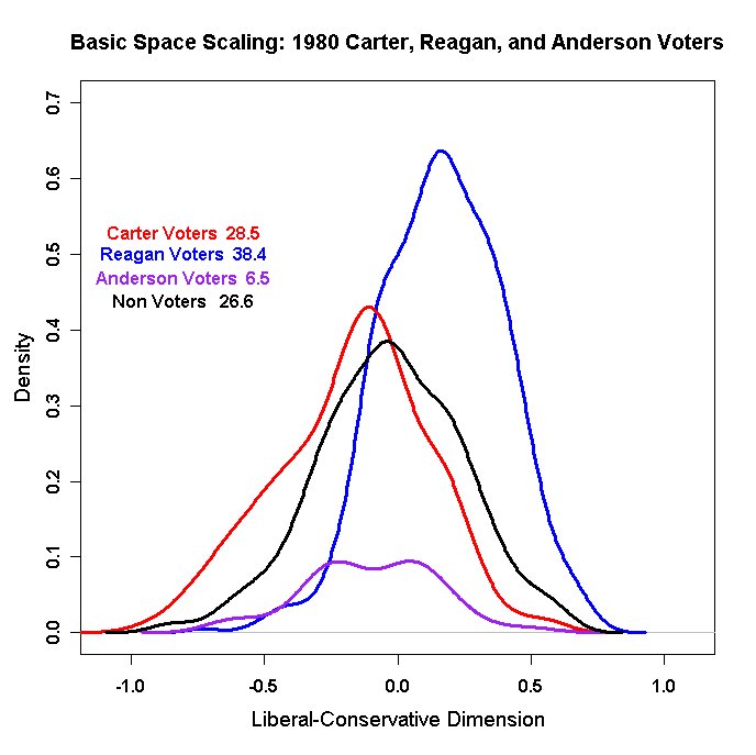
turn in this graph.
- Make separate two-dimensional plots of the Reagan, Carter, and Anderson voters and
non-Voters using the first two dimensions of the the 3-dimensional coordinates.