Measurement Theory Spring 2003: First Assignment Page

LEGACY CONTENT. If you are looking for Voteview.com, PLEASE CLICK HERE

This site is an archived version of Voteview.com archived from University of Georgia on May 23, 2017. This point-in-time capture includes all files publicly linked on Voteview.com at that time. We provide access to this content as a service to ensure that past users of Voteview.com have access to historical files. This content will remain online until at least January 1st, 2018. UCLA provides no warranty or guarantee of access to these files.

POLS 6386 MEASUREMENT THEORY
First Assignment
Due 28 January 2003

The aim of this problem is to familarize you with the classic KYST scaling program. Download the program

KYST Program

and the sample data file

KYST Supreme Court Data

and place them in the same folder on a WINTEL machine.

The sample data file is reproduced below. It contains the lower half of an agreement score matrix computed between the 31 supreme court justices who served on the court from 1945 to 2000.


TORSCA                   Method to get initial starting configuration
PRE-ITERATIONS=3         Number Iterations to Improve starting config.
DIMMAX=2,DIMMIN=1        Maximum & Minimum Number of Dimensions
COORDINATES=ROTATE       Rotate Coordinates so Principal Components lie along axes
ITERATIONS=25            Maximum Number of Iterations
REGRESSION=DESCENDING    Monotone Regression for Similarities -- NONMETRIC MDS
DATA,LOWERHALFMATRIX,DIAGONAL=PRESENT,CUTOFF=.01 Anything below .01 is Missing Data
U. S. SUPREME COURT AGREEMENT SCORES Title
 32  1  1                32 = # of Justices, Always set the next two numbers = 1
(12X,101F3.0)            Format Statement For Dataset
BURGER      100
BLACKMUN     81100
POWELL       86 80100
REHNQUIS     87 72 83100
STEVENS      71 77 74 67100
OCONNOR      88 72 86 87 71100
SCALIA      -99 66 85 89 65 85100
KENNEDY     -99 70-99 88 70 86 87100         -99 is the Missing Data Code
SOUTER      -99 72-99 78 75 81 77 84100
THOMAS      -99 55-99 86 56 81 92 82 72100
GINSBURG    -99 67-99 73 80 75 70 79 87 67100
BREYER      -99-99-99 70 78 77 64 75 84 63 84100
RUTLEDGE    -99-99-99-99-99-99-99-99-99-99-99-99100
MURPHY      -99-99-99-99-99-99-99-99-99-99-99-99 86100
VINSON      -99-99-99-99-99-99-99-99-99-99-99-99 63 64100
HARLAN       81 78-99-99-99-99-99-99-99-99-99-99-99-99-99100
BLACK        67 69-99-99-99-99-99-99-99-99-99-99 85 85 63 58100
DOUGLAS      39 42 42 33-99-99-99-99-99-99-99-99 78 79 59 50 77100
STEWART      77 75 80 74 75-99-99-99-99-99-99-99-99-99-99 78 67 58100
MARSHALL     54 65 57 46 65 51 50 50 53-99-99-99-99-99-99 70 66 70 69100
BRENNAN      53 64 56 46 65 52 51 52100-99-99-99-99-99-99 66 76 76 70 91100
WHITE        80 76 79 77 69 77 79 80 76 74-99-99-99-99-99 74 73 56 76 59 64100
WARREN      -99-99-99-99-99-99-99-99-99-99-99-99-99-99-99 60 81 79 71 90 91 79100
CLARK       -99-99-99-99-99-99-99-99-99-99-99-99-99-99 91 74 67 61 77-99 77 83 77100
FRANKFUR    -99-99-99-99-99-99-99-99-99-99-99-99 58 61 70 86 60 55 79-99 67-99 63 71100
WHITTAKE    -99-99-99-99-99-99-99-99-99-99-99-99-99-99-99 81 57 52 82-99 66-99 62 75 80100
BURTON      -99-99-99-99-99-99-99-99-99-99-99-99 62 58 83 77 60 56-99-99 65-99 66 81 72 80100
REED        -99-99-99-99-99-99-99-99-99-99-99-99 65 62 84 67 60 60-99-99 69-99 71 82 67-99 82100
FORTAS      -99-99-99-99-99-99-99-99-99-99-99-99-99-99-99 63 68 76 72 89 87 75 85 74-99-99-99-99100
GOLDBERG    -99-99-99-99-99-99-99-99-99-99-99-99-99-99-99 59 78 80 77-99 90 78 87 71-99-99-99-99-99100
MINTON      -99-99-99-99-99-99-99-99-99-99-99-99-99-99 87 72 62 57-99-99-99-99 75 84 68-99 82 83-99-99100
JACKSON     -99-99-99-99-99-99-99-99-99-99-99-99 57 57 75-99 57 53-99-99-99-99 75 78 80-99 74 73-99-99 73100
COMPUTE                 These two Lines             
STOP                    Must Always be Included

You must run the program from a DOS Window. To run the program type:

KYSTBIG

The program will then prompt you for three file names: the name of the data file (it calls this the "Control Card File"); the name of an output file that you can then print out; and the name of the file for the coordinates.

Control Card File? SUPKYST.DAT
Printer Output File? SUPREME.PRN
Coordinate Output File? SUPS.DAT

The program then runs the analysis and writes the output files to disk.

Produce graphs of the one and two dimensional coordinates that are in the SUPS.DAT.
Interpret the one dimensional configuration. In light of what you know about the Supreme Court does in make sense to you?

Download data file

U. S. Map Driving Distance Data

and place it in the same folder with KYST.

The data file is reproduced below. It contains the lower half of a driving distance matrix computed between 10 U.S. cities -- Atlanta, Boise, Boston, Chicago, Cincinnati, Dallas, Denver, Los Angeles, Miami, and Washington, D.C..
```
PRINT HISTORY, PRINT DISTANCES         This Option Prints out Some Useful Intermediate Output
DIMMAX=3, DIMMIN=1
TORSCA
REGRESSION=POLYNOMIAL=1                METRIC MDS
DATA,LOWERHALFMATRIX,DIAGONAL=PRESENT,CUTOFF=0.0
U.S. MAP EXAMPLE
 10  1  1
(10f5.0)
 0000
 2340 0000
 1084 2797 0000
  715 1789  976 0000
  481 2018  853  301 0000
  826 1661 1868  936  988 0000
 1519  891 2008 1017 1245  797 0000
 2252  908 3130 2189 2292 1431 1189 0000
  662 2974 1547 1386 1143 1394 2126 2885 0000
  641 2480  443  696  498 1414 1707 2754 1096 0000
COMPUTE
STOP
```
1. Run this data set through KYST and get the coordinates. Plot the coordinates in two dimensions. What do you see?
2. Change REGRESSION=POLYNOMIAL=1 to REGRESSION=ASCENDING and run it through KYST (the "ascending" tells KYST to do a Nonmetric MDS on dissimilarity data). Compare the Stress values for 1 to 3 dimensions with those obtained above and compare the two dimensional plot obtained with this option to that in part (a).
In this problem you are going to replicate the MCMC example on pages 26 - 29 of Gill.
- First, use Epsilon to type in the R code on page 28 of Gill. Be sure to enter the code exactly as written!
- Name the file Gill_1.R and place it in a directory, for example, d:\R_Files (or something you will remember).
- Start R
- Under the "File" Menu, select "Source R Code". You will get a standard WINDOWS directory-tree dialog box. Select the directory that you saved Gill_1.R in and click "open". R will think for a second and then you should see:
  
  source("D:/r_files/gill_1.r")
- To run the program type:
  
  run <- gill_1
  
  This runs the program in the background and generates the two vectors of numbers, x and y.
- To see the entries of x, type:
  
  x
  
  and the entries will appear on the screen. Your computer screen should look something like the following:
  
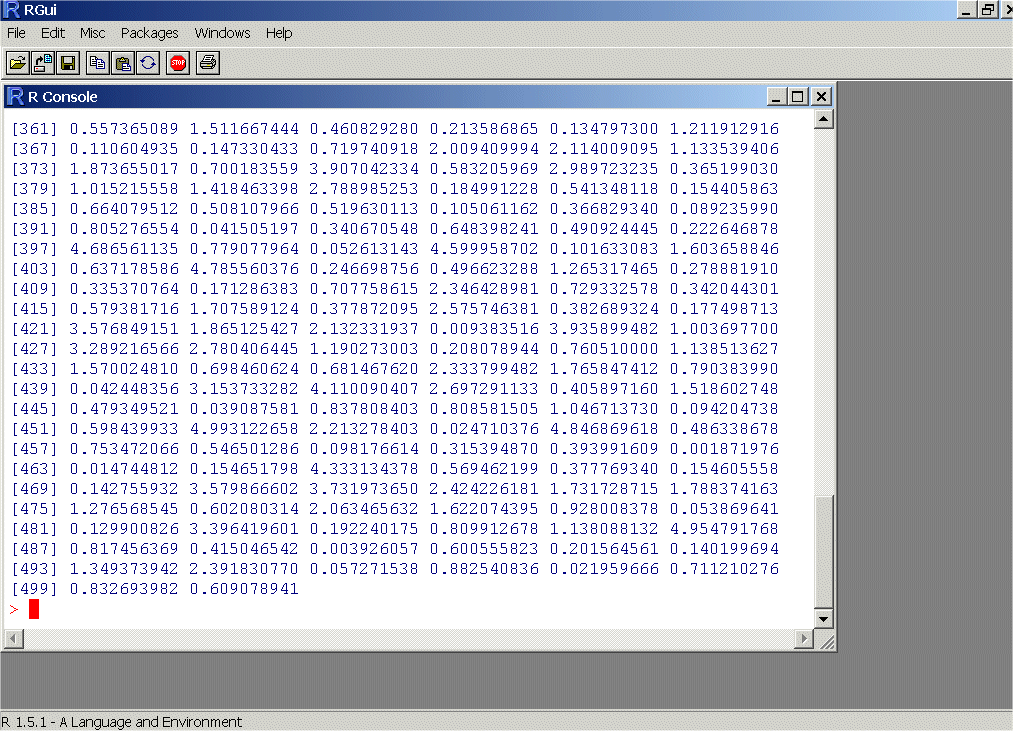
  Your numbers will look slightly different from mine because I tinkered with the computer code.
- It is always a good idea to keep a copy of everything you do in R! To do this, go to the "File" menu and select "Save to File". A standard WINDOWS file save dialog box comes up with a default file name of "lastsave" with default extension of "*.TXT". You can rename it to "Gill_1.Txt" if you like so you won't accidently overwrite it later.
- Open "Gill_1.Txt" with Epsilon. You should see everything that has appeared on the screen so far:
  
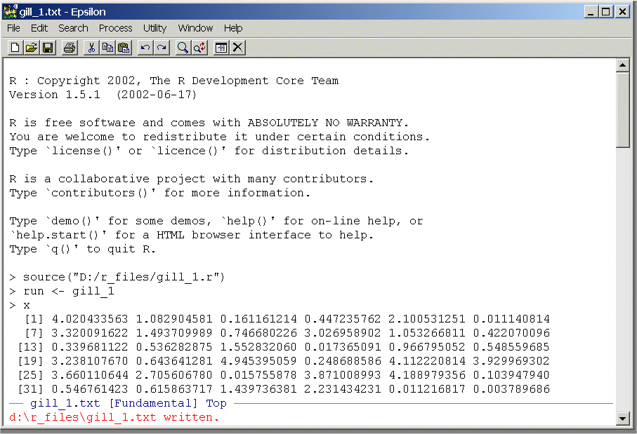
  This is extremely handy for obvious reasons!
- Go back to R and display the entries of y. Type:
  
  y
  
  and the entries will appear on the screen. Now, repeat the step above where you saved the screen contents to "Gill_1.Txt". Simply overwrite the previous version. Now go back to Epsilon and you will hear a "ding" and you should see this:
  
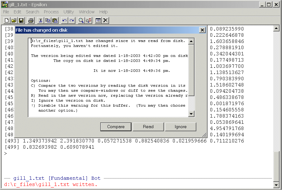
  Click "Read" and you should see this:
  
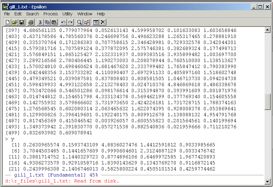
  Again, my numbers will be a bit different from yours.
- Now, lets replicate the histograms that Gill shows on page 29. To do this, use the command:
  
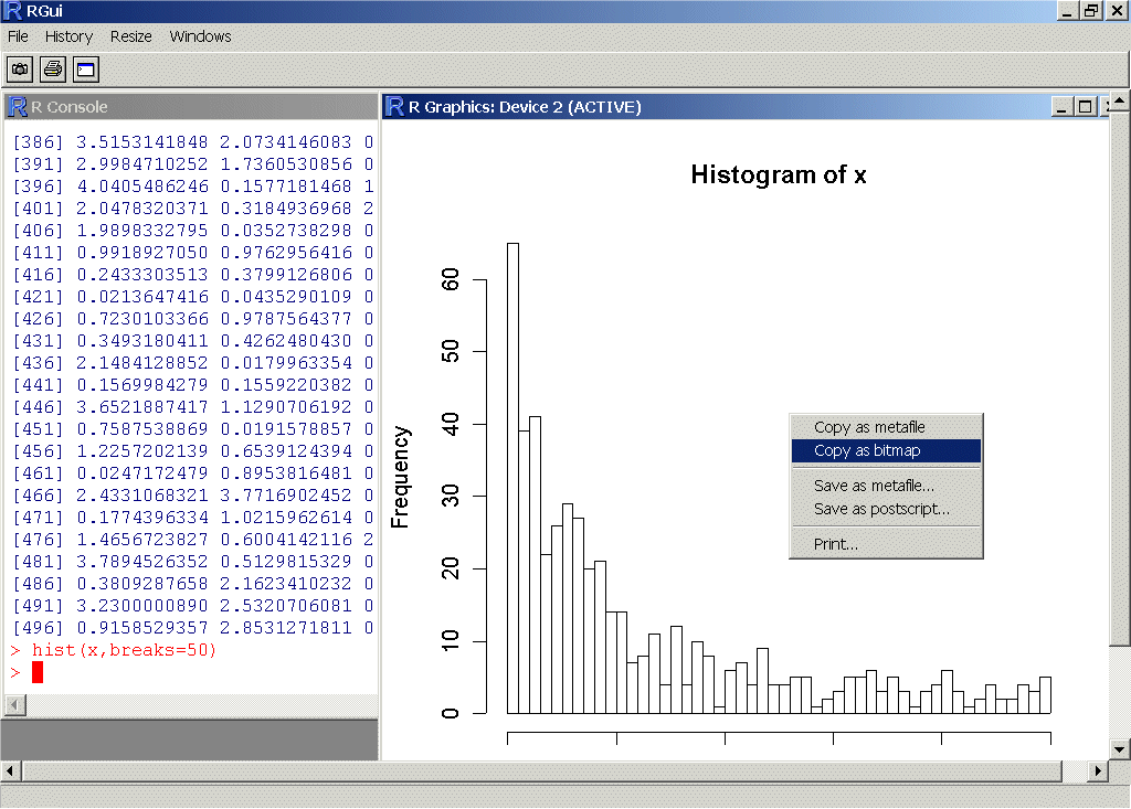
  hist(x,breaks=50)
  
  The "breaks=50" creates 50 bars. Now, right click on the image on the screen and select "copy as bitmap" (see below)
- Now you can go to WORD and simply paste the image into your document (see below):
  
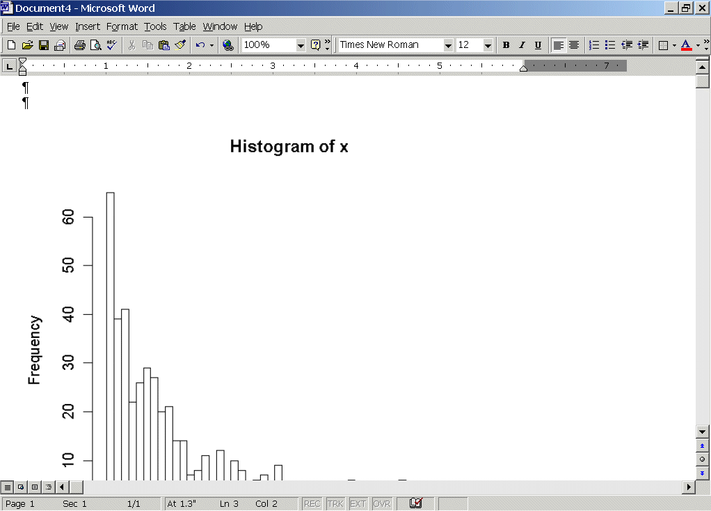
  (Note that its slightly cut off in the screen shot.)
1. Repeat this process for the vector y and turn in both graphs in WORD in your homework.
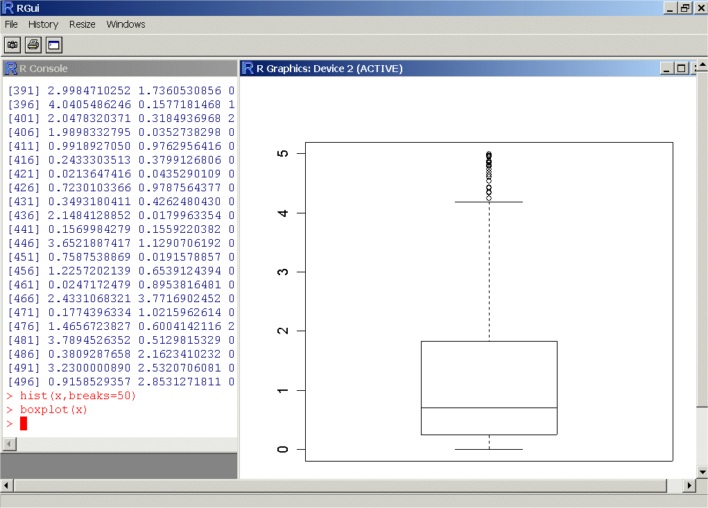
2. Produce a boxplot for both x and y. To do this in R type:
  
  boxplot(x)
  
  Your should see something like this:
  
  Repeat this for the variable y and paste both of these graphs into your homework answer.
3. Report the means and standard deviations of x and y. To do this, use the commands:
  
  mean(x)
  
  and
  
  sd(x)
4. Produce Histograms of both x and y with an exponential function overlay. To do this, first type the command:
  
  hist(x,freq=F)
  
  This produces a histogram. Minimize this picture so that the R command window has the focus (clicking on the R command window should bring it to the front as well). Now enter the command:
  
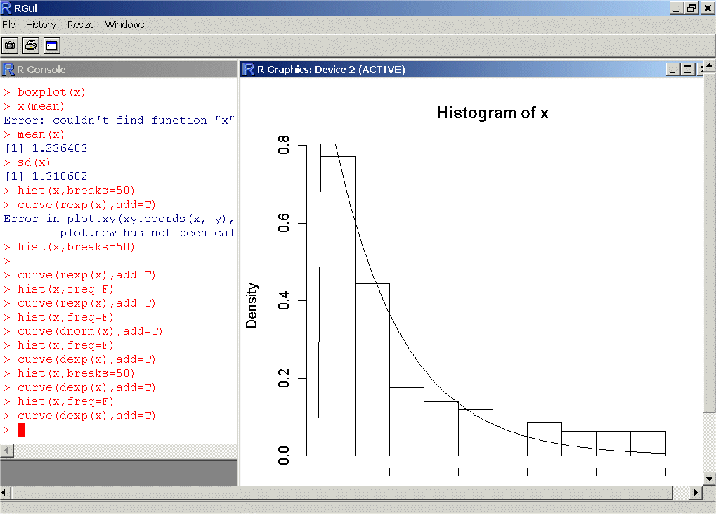
  curve(dexp(x),add=T)
  
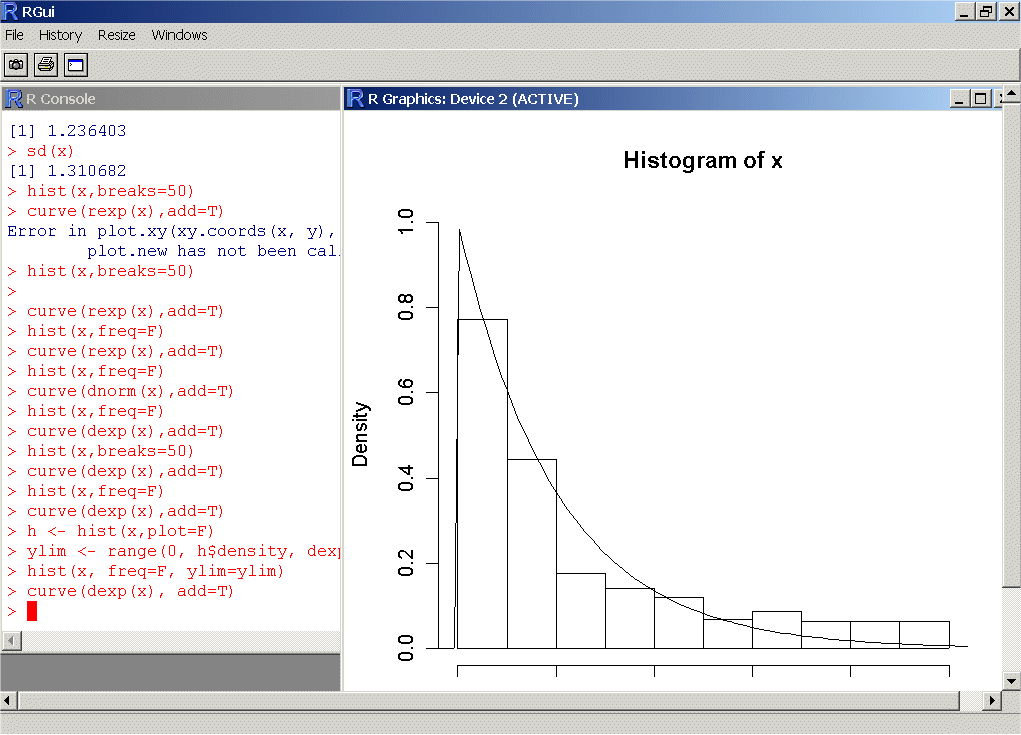
  This command tells R to plot the best fitting exponential curve over the top of the existing plot. You should see something that looks like this:
  
  Paste the plots for x and y into your homework answer.
5. The previous plot was a bit sloppy in that the top was cut off. To make better plots we need to tell R what the maximum value is for our exponential function. To do this, first enter the commands:
  
  h <- hist(x,plot=F)
  ylim <- range(0, h$density, dexp(0))
  
  The first command retrieves the bar heights and places them in the variable h (later, try typing h at the command prompt). The second command calculates the range for the bars and the overlying density. Note that dexp(0) is the exponential evaluated at zero -- the maximum value of the function.
  
  Now type:
  
  hist(x, freq=F, ylim=ylim)
  and the histogram will appear. Return the focus to the R command window and type:
  
  curve(dexp(x), add=T)
  
  You should see something like the following:
  
  Paste the plots for x and y into your homework answer.

DO NOT FORGET TO PERIODICALLY SAVE EVERYTHING YOU HAVE DONE AS I EXPLANED ABOVE!!!