POLS 6482 ADVANCED MULTIVARIATE STATISTICS
Second Assignment
Due 17 September 2001

As we discussed in class, turn in all of your output neatly formatted in WORD! Any command in STATA or EVIEWS that produces output -- regression tables, histograms, correlation matrices, etc. -- must be neatly pasted into your homework answer!

1. The aim of this problem is to investigate some simple relationships between party identification and a few social-economic characteristics. The data come from the 1968 and 1996 NES presidential election surveys. The variables are:

   
   
         Party Identification:  0=strong democrat
                                1=weak democrat
                                2=lean democrat
                                3=independent
                                4=lean republican
                                5=weak republican
                                6=strong republican
                                 
         Family Income Quintile:  1 is the lowest quintile, 5 is the highest
    
         Race:  0 = White
                1 = Black
   
         Sex:   0 = Male
   			      1 = Female
         
         South: 0 = North
                1 = South
   
         Education:  1 = High School or less
                     2 = Some College
                     3 = College degree
   
         Age:   In Years
   

   The data are in two text files:
   
   1968 Data
   1996 Data
   
   In order to do the assignment you need to download these two files one at a time and load them into EVIEWS. The first step is to download the files and place them on a disk (a floppy is fine). Now start EVIEWS and type:
   
   CREATE
   
   You will get the "Workfile Range" pop-up window. Select the "undated or irregular" option. The 1968 data set has 1585 observations and the 1996 data set has 1547 observations. If you are working with the 1968 data set type "1585" in the "End observation" window and click "OK". You will now see the pop-up window "Workfile: UNTITLED". Now you need to read the data into EVIEWS. Type:
   
   READ(o)
   
   [Note that the argument in READ() is "o" (oh), not "0" (zero)!] The standard windows file open pop-up window now appears and simply type in the path to OLS68.TXT/OLS96.TXT. You will now get the "ASCII Text Import" pop-up window in EVIEWS. The cursor will be positioned in the field "Names for series or Number of series if names in file". Type in the following for the variable names:
   
   party income race sex south education age
   
   and click "OK". You do not need to put commas between the names of the variables. Also, you need to enter the variable names in the same order as their corresponding columns in the data matrix!
   
   You will now see the EVIEWS "Workfile: UNTITLED" window with all the variable names. You should now save the workfile as NES68.WF1/NES96.WF1.
   
   After you have the first workfile entered and saved, to get the second data set into EVIEWS, simply go to the "File" menu and select "new" and then select "Workfile". You will get another workfile window with the label "Workfile: UNTITLED". Simply enter the command:
   
   READ(o)
   
   to get the second data set and go through the same steps described above.
   
   You now should have two workfiles in EVIEWS: NES68 and NES96.
   
   We are now going to test the following political theory:
   
   Party = f(income, race, sex, south, education, age)
   
   or, expressed in terms of a regression equation:
   
   y = b₀ + b₁x₁ + b₂x₂ + b₃x₃ + b₄x₄ + b₅x₅ + b₆x₆ + e
   
   where y = party, x₁ = income, x₂ = race, x₃ = sex, x₄ = south, x₅ = education, and x₆ = age.
   
   
   1. Ignoring the constant term -- b₀ -- what should be the signs on the coefficents in the equation? Why? Justify your answer. For example, the dependent variable, party, ranges from 0 (strong democrat) to 6 (strong republican) and the variable income ranges from 1 (lowest income quintile) to 5 (highest income quintile). Hence, a reasonable assumption is that the coefficient on income, b₁, should be positive (b₁ > 0).
      
      
   2. Run the above regression for both elections. The EVIEWS command is:
      
      LS Party C Income Race Sex South Education Age
      
      Generally speaking, if the P-Value ("Prob." column in the EVIEWS regression table) is greater than .20 we can conclude that, ceteris paribus, that the variable is not substantively important. Traditionally, for statistical significance, a value of .10 is required.
      
      
   3. Interpret the results in light of your beliefs on the signs of the coefficients and compare the pattern of the coefficents for 1968 and 1996. What do you think are the important changes? Do these changes make sense to you?
      
      
2. The aim of this problem is to learn to transfer a dataset from EVIEWS to STATA. To do this, start STATA and open up the data editor. It should look like this:
   
   
   
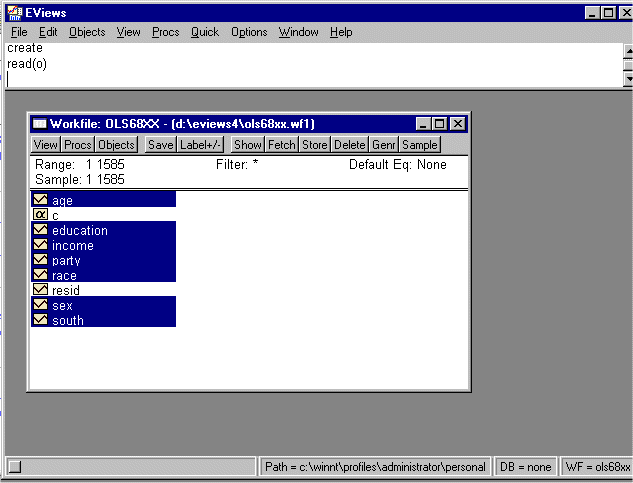
   Go back to EVIEWS and click the "view" button on the Workfile toolbar and click on the option "Select All (except C-RESID)". You should see the following:
   
   
   
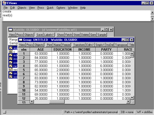
   Double click on the highlighted variables and they will come up in a spreadsheet format. (In EVIEWS 4.0 a gray dialog box will pop up first. Select "open group" and the spreadsheet comes up.) You should see the following:
   
   
   
   Highlight the entries of the spreadsheet and place them on the clipboard. You will get the following prompt:
   
   
   
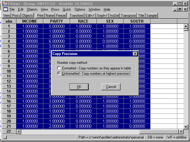
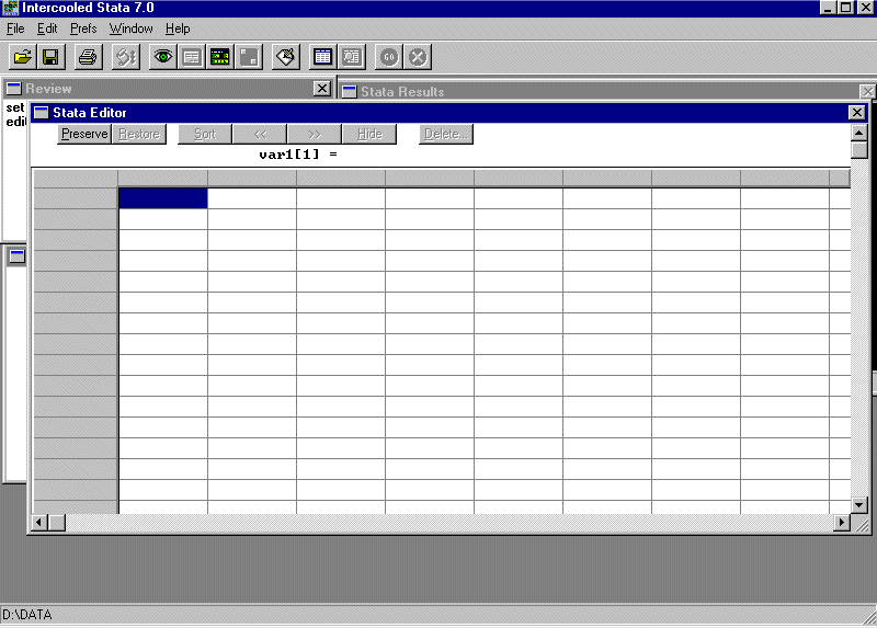
   Select the "highest precision" option. Now, go into STATA and paste the spreadsheet into the data editor. You will see:
   
   
   
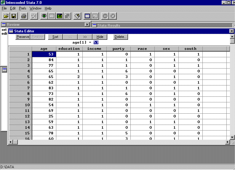
   Now insert definitions of the variables into the STATA spreadsheet (see first homework). Use the definitions in (1) above (you can use abbreviations, etc.)
   
   
   1. Do the d and summ commands for both the 1968 and 1996 datasets and paste the results into your homework answer.
      
      
   2. Replicate the regressions in STATA that you ran in EVIEWS for both the 1968 and 1996 datasets. In STATA, enter the command:
      
      regress party income race sex south education age
      
      
3. The aim of this problem is to familarize you with eigenvalues and eigenvectors of a correlation matrix and some handy features in EVIEWS.
   
   Bring up EVIEWS and open a new workfile. Select the "undated or irregular" option and set the number of observations to 1000. You are going to create a number of variables by drawing randomly from a Normal Distribution. Enter the command:
   
   GENR X1=NRND
   
   This creates a 1000 length vector consisting of random draws from the Normal Distribution with Mean 0 and Variance 1. To check this use the "Histogram and Stats" option under "series statistics" on the "Quick" option of the menu bar (you did this in homework one). You can also type:
   
   HIST X1
   
   Now enter the following commands:
   
   GENR X2=2*(NRND-1)
   
   GENR X3=2*NRND-1
   
   GENR X4=(1/3)*NRND
   
   
   1. Verify (use the HIST command) that the means and standard deviations are -2, 2; -1, 2; and 0, 1/3; respectively.
      
      
   2. Compute the correlation matrix with the command:
      
      COR X1 X2 X3 X4
      
      What should the values of these correlations be? Why?
      
      
   3. Now we are going to compute the eigenvalues and eigenvectors of the correlation matrix. To do this, enter the commands:
      
      group g1 x1 x2 x3 x4
      matrix m1=g1
      sym corrmat=@cor(m1)
      vector eigenvalue=@eigenvalues(corrmat)
      matrix eigenvectors=@eigenvectors(corrmat)
      show eigenvalue
      show eigenvectors
      
      The last two commands simply show the results on the screen. Add the eigenvalues -- what do they add up to?