POLS 6482 ADVANCED MULTIVARIATE STATISTICS
Seventh Assignment
Due 22 October 2001

1. This problem is a simple exercise with dummy variables. The data are discussed on pages VII-2 to VII-8 of the Epple notes. The data file is:
   
   Package Delivery Data
   
   
   1. Replicate the analyses shown in the Epple notes using EVIEWS. Use the @FDIST(_,_,_) command to get the exact P-Value for the test discussed on VII-8.
      
      
   2. In EVIEWS, run the following regression:
      
      LS mins 1-dum dum delivs
      
      and compare the results with:
      
      LS mins C dum delivs
      
      How are the two different? Why?
      
      
   3. Paste the data into STATA and replicate the analyses in parts (a) and (b). In STATA, you can get the p-value with the command (see homework 5):
      
      display fprob(_,_,_)
      
      In STATA you can suppress the constant (intercept) term with the command:
      
      regress mins dum2 dum delivs, hascons
      
      (dum2 = 1 - dum)
      
      hascons tells STATA that the independent variables incorporate the constant! To see the difference, try the command:
      
      regress mins dum2 dum delivs, nocons
      
      
   4. What is the difference between the two outputs?
      
      
2. This problem deals with the awards in wrongful death cases. This dataset is discussed in Epple Notes VI-36 to VI-41 and VII-10 to VII-14.
   
   Awards in Wrongful Death Court Cases
   
   
   1. Download the dataset and replicate the analyses shown in Epple Notes VI-36 to VI-40.
      
      
   2. Answer the two questions on VI-40 about a unit change in income and the slope of the relationship between award and earnings.
      
      
   3. There are several dummy (indicator) variables included in the dataset. With respect to the regression results shown on page VI-38, what is the omitted category that is being picked up by the intercept term?
      
      
   4. With respect to (c), re-run the regression with the omitted indicator variable (don't use C!). Do the coefficients have the correct values?
      
      
   5. Run the Ramsey RESET Test with one, two, and three fitted terms (see Epple Notes VI-13 to VI-16). Do the results make sense to you?
      
      
   6. Perform the four tests discussed on page VII-12 (Q7.2 - Q7.5). Use the specification with age interacted with earnings. Under the View button on the regression table, select Representations and report the results so that your Wald Tests are clearly reported. The Representations command should produce something that looks like this:
      

      Estimation Command:
      =====================
      LS AWARD C AGE AREAPI CHILD CORP DATE EARN GOVT JURY SMLBIZ AGE*EARN
      
      Estimation Equation:
      =====================
      AWARD = C(1) + C(2)*AGE + C(3)*AREAPI + C(4)*CHILD + C(5)*CORP + C(6)*DATE + C(7)*EARN + 
              C(8)*GOVT + C(9)*JURY + C(10)*SMLBIZ + C(11)*(AGE*EARN)
      
      Substituted Coefficients:
      =====================
      AWARD = -219.7246158 - 0.6092463913*AGE + 0.006719394952*AREAPI + 20.42366783*CHILD + 
                63.02345024*CORP + 12.01049539*DATE + 10.72571602*EARN + 184.5738731*GOVT + 
               131.2040308*JURY + 67.237274*SMLBIZ - 0.1172755132*(AGE*EARN)
      

      With respect to the last test -- whether or not governments, corporations, and small businesses pay the same amount -- discuss its political significance.
      
      
   7. Paste the dataset into STATA, define the variables appropriately, and turn in the d and summ commands. Replicate the regressions and tests discussed in (c) - (f). To perform the Ramsey RESET Test in STATA, run the regression and then use the command:
      
      ovtest
      
      Note that STATA automatically uses three fitted values.
      
      To perform the coefficient tests use the test command described in the 5^th Homework. For example, to test the null hypothesis that the amount paid by corporations is the same as that paid by small business:
      
      test corp=smlbiz
      
      and STATA will respond with
      

      
      
       ( 1)  corp - smlbiz = 0.0
      
             F(  1,   161) =    0.02
                  Prob > F =    0.8900
      

   8. Graph the residuals against the fitted values. In STATA, you can do this with the command:
      
      rvfplot, border yline(0)
      
      rvfplot stands for "residual-versus-fitted plot", border draws a line around the graph, and yline(0) draws a line across the graph at y = 0.
      
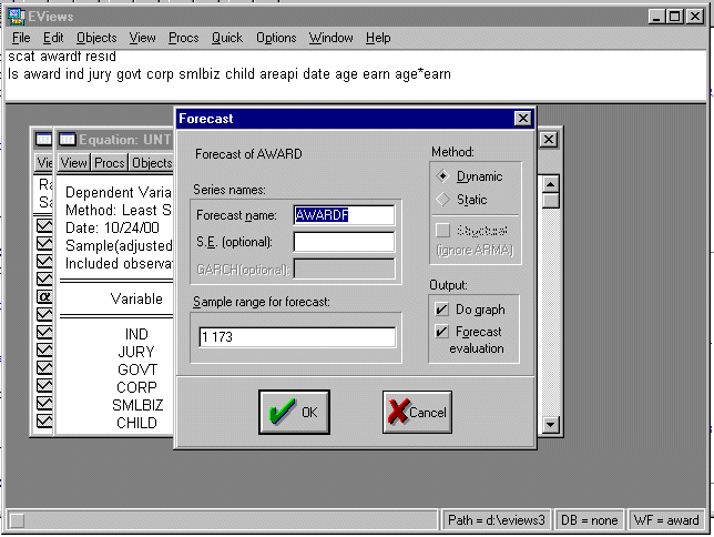
      In EVIEWS, to generate the same graph run the regression and then click on the Forecast button. You will see:
      
      
      
      Click OK and you will see a graph (note that you can turn off that option). Kill the graph and you will see AWARDF as one of the variables in the workfile window. To get the graph use the command
      
      scat awardf resid
      
      In EVIEWS, try the commands:
      
      scat(R) awardf resid
      
      and scat(R) award awardf
      
      the "(R)" puts in a regression line. What is your interpretation of these two graphs?