- In this problem we are going to analyze Eckman's famous color circle data.
Use the R program below to do this exercise:
 Double_Center_Color_Circle.r -- Program to
Double-Center a Matrix of Squared Distances
Double_Center_Color_Circle.r -- Program to
Double-Center a Matrix of Squared Distances
#
#
# double_center_color_circle.r -- Double-Center Program
#
# Data Must Be Transformed to Squared Distances Below
#
#      **************** The Eckman Color Data *****************
#
# 434 INDIGO        100  86  42  42  18   6   7   4   2   7   9  12  13  16
# 445 BLUE           86 100  50  44  22   9   7   7   2   4   7  11  13  14
# 465                42  50 100  81  47  17  10   8   2   1   2   1   5   3
# 472 BLUE-GREEN     42  44  81 100  54  25  10   9   2   1   0   1   2   4
# 490                18  22  47  54 100  61  31  26   7   2   2   1   2   0
# 504 GREEN           6   9  17  25  61 100  62  45  14   8   2   2   2   1
# 537                 7   7  10  10  31  62 100  73  22  14   5   2   2   0
# 555 YELLOW-GREEN    4   7   8   9  26  45  73 100  33  19   4   3   2   2
# 584                 2   2   2   2   7  14  22  33 100  58  37  27  20  23
# 600 YELLOW          7   4   1   1   2   8  14  19  58 100  74  50  41  28
# 610                 9   7   2   0   2   2   5   4  37  74 100  76  62  55
# 628 ORANGE-YELLOW  12  11   1   1   1   2   2   3  27  50  76 100  85  68
# 651 ORANGE         13  13   5   2   2   2   2   2  20  41  62  85 100  76
# 674 RED            16  14   3   4   0   1   0   2  23  28  55  68  76 100
#
#
#  Remove all objects just to be safe
#
rm(list=ls(all=TRUE))
#
library(MASS)
library(stats)
#
#
rcx.file <- "c:/ucg_course_homework_8/color_circle.txt"
#
# Standard fields and their widths
#
rcx.fields <- c("colorname","x1","x2","x3","x4","x5",
                   "x6","x7","x8","x9","x10","x11","x12","x13","x14")
rcx.fieldWidths <- c(18,4,4,4,4,4,4,4,4,4,4,4,4,4,4)
#
# Read the vote data from fwf
#
U <- read.fwf(file=rcx.file,widths=rcx.fieldWidths,as.is=TRUE,col.names=rcx.fields)
dim(U)
ncolU <- length(U[1,])   Note the "trick" I used here
T <- U[,2:ncolU]           The 1st column of U has the color names
#
#
nrow <- length(T[,1])
ncol <- length(T[1,])
#           Even though I have the color names in U this is more convenient
#             because there are no leading or trailing blanks
names <- c("434 Indigo","445 Blue","465","472 Blue-Green","490","504 Green","537",
           "555 Yellow-Green","584","600 Yellow","610","628 Orange-Yellow",
           "651 Orange","674 Red")
#
# pos -- a position specifier for the text. Values of 1, 2, 3 and 4,
# respectively indicate positions below, to the left of, above and
# to the right of the specified coordinates
#
namepos <- rep(2,nrow)
#
TT <- rep(0,nrow*ncol)
dim(TT) <- c(nrow,ncol)
TTT <- rep(0,nrow*ncol)
dim(TTT) <- c(nrow,ncol)
#
xrow <- NULL
xcol <- NULL
xcount <- NULL
matrixmean <- 0
matrixmean2 <- 0
#
# Transform the Matrix
#
#
#  Transform the Color "Agreement Scores" into Distances
#
     TT <- ((100-T)/50)**2   Note the Transformation from a 100 to 0 scale
#                             to a 0 to 4 (squared distance) scale
#  Put it Back in T
#
T <- TT
TTT <- sqrt(TT)
#
#
#  Call Double Center Routine From R Program
#     cmdscale(....) in stats library
#     The Input data are DISTANCES!!!  Not Squared Distances!!
#     Note that the R routine does not divide
#     by -2.0
#
ndim <- 2
#
dcenter <- cmdscale(TTT,ndim, eig=FALSE,add=FALSE,x.ret=TRUE)
#
#  returns double-center matrix as dcenter$x if x.ret=TRUE
#
#  Do the Division by -2.0 Here
#
TTT <- (dcenter$x)/(-2.0)
#
#
#  Below is the old Long Method of Double-Centering
#
# Compute Row and Column Means
#
i <- 0
while (i < nrow) {
  i <- i + 1
  xrow[i] <- mean(T[i,])
}
i <- 0
while (i < ncol) {
  i <- i + 1
  xcol[i] <- mean(T[,i])
}
matrixmean <- mean(xcol)
matrixmean2 <- mean(xrow)
#
# Double-Center the Matrix Using old Long Method
#  Compute comparison as safety check
#
i <- 0
while (i < nrow) {
  i <- i + 1
  j <- 0
  while (j < ncol) {
     j <- j + 1
     TT[i,j] <- (T[i,j]-xrow[i]-xcol[j]+matrixmean)/(-2)
  }
}
#
#  Run some checks to make sure everything is correct
#
xcheck <- sum(abs(TT-TTT))
#
#
#  Perform Eigenvalue-Eigenvector Decomposition of Double-Centered Matrix
#
ev <- eigen(TT)
#
#  Find Point furthest from Center of Space
#
aaa <- sqrt(max((abs(ev$vec[,1]))**2 + (abs(ev$vec[,2]))**2))
bbb <- sqrt(max(((ev$vec[,1]))**2 + ((ev$vec[,2]))**2))
#
#  Weight the Eigenvectors to Scale Space to Unit Circle
#
torgerson1 <- ev$vec[,1]*(1/aaa)*sqrt(ev$val[1])
torgerson2 <- -ev$vec[,2]*(1/aaa)*sqrt(ev$val[2])
#
plot(torgerson1,torgerson2,type="n",asp=1,
       main="",
       xlab="",
       ylab="",
       xlim=c(-3.0,3.0),ylim=c(-3.0,3.0),font=2)
points(torgerson1,torgerson2,pch=16,col="red",font=2)
text(torgerson1,torgerson2,names,pos=namepos,offset=0.2,col="blue",font=2)
#
#
# Main title
mtext("The Color Circle \n Torgerson Coordinates",side=3,line=1.25,cex=1.5,font=2)
# x-axis title
mtext("",side=1,line=2.75,cex=1.2,font=2)
# y-axis title
mtext("",side=2,line=2.5,cex=1.2,font=2)
#
Run the program and you should see something like this:
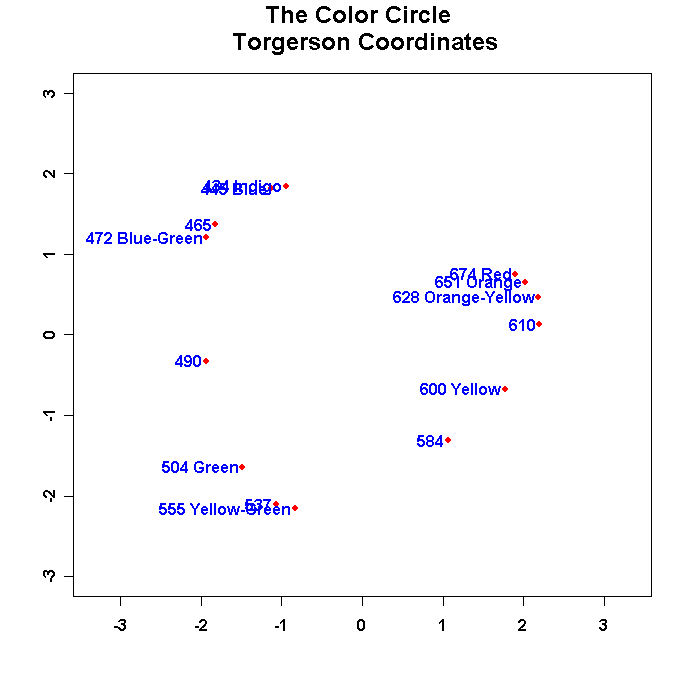
- Run the program and turn in this figure.
- Change the values in "namepos" until you have a nice looking plot with no overlapping
names and no names cut off by the margins and turn in the resulting plot. Use the offset
parameter in the text command to space the names away from the points. Also
flip the dimensions as appropriate so that the configuration matches the one
in Borg and Goenen!
- Check out:
Color Circle in Color
Use the colors() command in
R to find the corresponding colors and
then use the text command to color the label for the corresponding point; e.g.,
text(torgerson1[10],torgerson2[10],"Yellow",pos=4,col="yellow",font=2)
You will have to override the labeling command in the double-center program to do this. Turn in
the plot (hard copy in B/W and e-mail it to me so I can see it!)
and the listing of
your R program.
- Plot the eigenvalues that are stored in ev$value.
- In this problem we are going to analyze Eckman's famous color circle data
with the KYST program in R.
Use the R program below to do this exercise:
NonMetric_MDS_Color_Circle.r -- Program to
run non-metric MDS on the Color Circle Data
#
# NonMetric_MDS_color_circle.r -- NonMetric MDS Program
#
#
#      **************** The Eckman Color Data *****************
#
# 434 INDIGO        100  86  42  42  18   6   7   4   2   7   9  12  13  16
# 445 BLUE           86 100  50  44  22   9   7   7   2   4   7  11  13  14
# 465                42  50 100  81  47  17  10   8   2   1   2   1   5   3
# 472 BLUE-GREEN     42  44  81 100  54  25  10   9   2   1   0   1   2   4
# 490                18  22  47  54 100  61  31  26   7   2   2   1   2   0
# 504 GREEN           6   9  17  25  61 100  62  45  14   8   2   2   2   1
# 537                 7   7  10  10  31  62 100  73  22  14   5   2   2   0
# 555 YELLOW-GREEN    4   7   8   9  26  45  73 100  33  19   4   3   2   2
# 584                 2   2   2   2   7  14  22  33 100  58  37  27  20  23
# 600 YELLOW          7   4   1   1   2   8  14  19  58 100  74  50  41  28
# 610                 9   7   2   0   2   2   5   4  37  74 100  76  62  55
# 628 ORANGE-YELLOW  12  11   1   1   1   2   2   3  27  50  76 100  85  68
# 651 ORANGE         13  13   5   2   2   2   2   2  20  41  62  85 100  76
# 674 RED            16  14   3   4   0   1   0   2  23  28  55  68  76 100
#
#
#  Remove all objects just to be safe
#
rm(list=ls(all=TRUE))
#
library(MASS)
library(stats)
#
#
rcx.file <- "c:/uga_course_homework_8/color_circle.txt"
#
# Standard fields and their widths
#
rcx.fields <- c("colorname","x1","x2","x3","x4","x5",
                   "x6","x7","x8","x9","x10","x11","x12","x13","x14")
rcx.fieldWidths <- c(18,4,4,4,4,4,4,4,4,4,4,4,4,4,4)
#
# Read the vote data from fwf
#
U <- read.fwf(file=rcx.file,widths=rcx.fieldWidths,as.is=TRUE,col.names=rcx.fields)
dim(U)
ncolU <- length(U[1,])
T <- U[,2:ncolU]
TT <- ((100-T)/50)^2      Here is the Transformation into Squared Distances
T <- TT
#
nrow <- length(T[,1])
ncol <- length(T[1,])
#
names <- c("434 Indigo","445 Blue","465","472 Blue-Green","490","504 Green","537",
           "555 Yellow-Green","584","600 Yellow","610","628 Orange-Yellow",
           "651 Orange","674 Red")
#
# pos -- a position specifier for the text. Values of 1, 2, 3 and 4,
# respectively indicate positions below, to the left of, above and
# to the right of the specified coordinates
#
namepos <- rep(2,nrow)
#
#  The KYST routine does not like zero distances in the off-diagonal!!!
#     Do Error Catch here if necessary
#                                         This Error Catch is Necessary if
# If T[i,j] = 0 set TT[i,j] = .03           you have an off-diagonal term that is 0.0
#             else if set TT[i,j] = T[i,j]
#
#TT <- ifelse(T==0,0.03,T)
#
#
#  Call Classical Kruskal-Young-Shepard-Torgerson Non-Metric
#           Multidimensional Scaling Program
#
# TT -- Input
# kdim=2 -- number of dimensions
# y -- starting configuration (generated internally)
#
kdim <- 2
y <- rep(0,kdim*nrow)           The R routine is fussy about wanting
dim(y) <- c(nrow,kdim)            y to be a declared matrix!
#
wandrnmds <- isoMDS(TT,y=cmdscale(TT,kdim),kdim, maxit=50)
#
xmax <- c(wandrnmds$points[,1],wandrnmds$points[,2])
axismax <- max(abs(xmax))
#
#  ############################################
#  Flip Signs of Dimensions as Necessary Here
#  ############################################
#
xx <- -wandrnmds$points[,1]
yy <- -wandrnmds$points[,2]
#
#
plot(xx,yy,type="n",asp=1,
       main="",
       xlab="",
       ylab="",
       xlim=c(-axismax,axismax),ylim=c(-axismax,axismax),font=2)
#
text(-axismax+.10,axismax,paste("Stress = ",                 This is a nifty way to plot
                0.01*round(wandrnmds$stress, 2)),col="purple",cex=1.2) the Stress Value
#                                                            R Puts Stress out as a Percentage
#
points(xx,yy,pch=16,col="red",font=2)
text(xx,yy,names,pos=namepos,offset=0.2,col="blue",font=2)
#
#
# Main title
mtext("The Color Circle \nFrom NonMetric MDS in R",side=3,line=1.25,cex=1.5,font=2)
# x-axis title
mtext("",side=1,line=2.75,cex=1.2,font=2)
# y-axis title
mtext("",side=2,line=2.5,cex=1.2,font=2)
#
- Tidy up the plot so it looks nice by changing the values in namepos accordingly.
- Use Epsilon to change the number of dimensions
and run the program in 1, 3, 4, and 5 dimensions. Plot the Stress values for 1 - 5 dimensions
in the same fashion as you plotted the eigenvalues in previous problems.
- Continuing with the color circle data, we are going to read in starting
coordinates for the KYST program in R.
Use the R program below to do this exercise:
NonMetric_MDS_Color_Circle_2.r -- Program to
run non-metric MDS on the Color Circle Data
The two R programs are essentially the same except for the extra read of
the color coordinates themselves:#
# NonMetric_MDS_color_circle_2.r -- NonMetric MDS Program
#
#
# **************** The Eckman Color Data *****************
#
# 434 INDIGO 100 86 42 42 18 6 7 4 2 7 9 12 13 16
# 445 BLUE 86 100 50 44 22 9 7 7 2 4 7 11 13 14
# 465 42 50 100 81 47 17 10 8 2 1 2 1 5 3
# 472 BLUE-GREEN 42 44 81 100 54 25 10 9 2 1 0 1 2 4
# 490 18 22 47 54 100 61 31 26 7 2 2 1 2 0
# 504 GREEN 6 9 17 25 61 100 62 45 14 8 2 2 2 1
# 537 7 7 10 10 31 62 100 73 22 14 5 2 2 0
# 555 YELLOW-GREEN 4 7 8 9 26 45 73 100 33 19 4 3 2 2
# 584 2 2 2 2 7 14 22 33 100 58 37 27 20 23
# 600 YELLOW 7 4 1 1 2 8 14 19 58 100 74 50 41 28
# 610 9 7 2 0 2 2 5 4 37 74 100 76 62 55
# 628 ORANGE-YELLOW 12 11 1 1 1 2 2 3 27 50 76 100 85 68
# 651 ORANGE 13 13 5 2 2 2 2 2 20 41 62 85 100 76
# 674 RED 16 14 3 4 0 1 0 2 23 28 55 68 76 100
#
#
# Remove all objects just to be safe
#
rm(list=ls(all=TRUE))
#
library(MASS)
library(stats)
#
#
rcx.file <- "c:/uga_course_homework_8/color_circle.txt"
#
# Standard fields and their widths
#
rcx.fields <- c("colorname","x1","x2","x3","x4","x5",
"x6","x7","x8","x9","x10","x11","x12","x13","x14")
rcx.fieldWidths <- c(18,4,4,4,4,4,4,4,4,4,4,4,4,4,4)
#
# Read the vote data from fwf
#
U <- read.fwf(file=rcx.file,widths=rcx.fieldWidths,as.is=TRUE,col.names=rcx.fields)
dim(U)
ncolU <- length(U[1,])
T <- U[,2:ncolU]
TT <- ((100-T)/50)^2
T <- TT
#
nrow <- length(T[,1])
ncol <- length(T[1,])
#
rcx.file <- "c:/uga_course_homework_8/color_coords.txt"
# Here is the extra read --
# Standard fields and their widths Starting Coordinates are read in
#
rcx.fields <- c("colorname2","xx1","xx2")
rcx.fieldWidths <- c(19,7,7)
#
# Read the vote data from fwf
#
UU <- read.fwf(file=rcx.file,widths=rcx.fieldWidths,as.is=TRUE,col.names=rcx.fields)
dim(UU)
ncolUU <- length(UU[1,])
y <- as.matrix(UU[,2:ncolUU]) Note this -- R can be funny about
# data types
names <- c("434 Indigo","445 Blue","465","472 Blue-Green","490","504 Green","537",
"555 Yellow-Green","584","600 Yellow","610","628 Orange-Yellow",
"651 Orange","674 Red")
#
# pos -- a position specifier for the text. Values of 1, 2, 3 and 4,
# respectively indicate positions below, to the left of, above and
# to the right of the specified coordinates
#
namepos <- rep(2,nrow)
#
# The KYST routine does not like zero distances in the off-diagonal!!!
# Do Error Catch here if necessary
#
# If T[i,j] = 0 set TT[i,j] = .03
# else if set TT[i,j] = T[i,j]
#
#TT <- ifelse(T==0,0.03,T)
#
#
# Call Classical Kruskal-Young-Shepard-Torgerson Non-Metric
# Multidimensional Scaling Program
#
# TT -- Input
# kdim=2 -- number of dimensions
# y -- starting configuration (generated internally)
#
kdim <- 2
#y <- rep(0,kdim*nrow)
#dim(y) <- c(nrow,kdim)
#
wandrnmds <- isoMDS(TT,y,kdim, maxit=50) Contrast this with the previous version
#
xmax <- c(wandrnmds$points[,1],wandrnmds$points[,2])
axismax <- max(abs(xmax))
#
# ############################################
# Flip Signs of Dimensions as Necessary Here
# ############################################
#
xx <- -wandrnmds$points[,1]
yy <- -wandrnmds$points[,2]
#
#
plot(xx,yy,type="n",asp=1,
main="",
xlab="",
ylab="",
xlim=c(-axismax,axismax),ylim=c(-axismax,axismax),font=2)
#
text(-axismax+.10,axismax,paste("Stress = ",
0.01*round(wandrnmds$stress, 2)),col="purple",cex=1.2)
#
#
points(xx,yy,pch=16,col="red",font=2)
text(xx,yy,names,pos=namepos,offset=0.2,col="blue",font=2)
#
#
# Main title
mtext("The Color Circle \nFrom NonMetric MDS in R",side=3,line=1.25,cex=1.5,font=2)
# x-axis title
mtext("",side=1,line=2.75,cex=1.2,font=2)
# y-axis title
mtext("",side=2,line=2.5,cex=1.2,font=2)
#
- Tidy up the plot so it looks nice by changing the values in namepos accordingly.
- Here is what the coordinate file looks like:
 434 INDIGO         -0.317  0.902
 445 BLUE           -0.368  0.818
 465                -0.900  0.566
 472 BLUE-GREEN     -0.965  0.503
 490                -0.988 -0.133
 504 GREEN          -0.828 -0.650
 537                -0.547 -0.862
 555 YELLOW-GREEN   -0.310 -0.977
 584                 0.562 -0.736
 600 YELLOW          0.830 -0.389
 610                 1.026 -0.074
 628 ORANGE-YELLOW   1.006  0.227
 651 ORANGE          0.914  0.346
 674 RED             0.885  0.459
Use Epsilon to arbitrarily change some of the
coordinates and run the program to see if you get back the same Stress value.
Do this 5 times and turn in each plot and each set of starting coordinates.
- In this problem we are going to analyze the color similarities data
with a more realistic Likelihood Function where we assume that the
observed distances have a log-normal distribution. We are also
going to take a Bayesian approach and state prior distributions for
all of the parameters of our model. Hence, rather than minimizing
a squared-error loss function we are going to maximize the
log-likelihood of a posterior distribution
(see Question 1 of Homework 6). We are going to use a version of
metric_mds_nations_ussr_usa.r
which we used in Homeword 5, Question 3 to find
the coordinates and the variance term that maximizes
the log-liklihood of the posterior distribution.
Download the R program:
metric_mds_colors_log_normal.r
-- Program to optimize the Log-Normal Bayesian Model for the Colors Similarities data.
colors.txt
-- Colors Data used by metric_mds_colors_log_normal.r
Here is the function that computes the log-likelihood:
fr <- function(zzz){
#
xx[1:8] <- zzz[1:8]         There are 26 parameters: 14*2=28-3+1=26
xx[9:10] <- 0.0             The 14 points in 2 dimensions = 28 coordinates
xx[11:19] <- zzz[9:17]      The 5th point -- 490 Angstroms is the origin and
xx[20] <- 0.0                the 2nd Dimension of 600 Angstroms is set to 0.0
xx[21:28] <- zzz[18:25]     Hence, 25 coordinates plus the variance term = 26 parameters
sigmasq <- zzz[26]
kappasq <- 100.0
sumzsquare <- sum(zzz[1:25]**2)
#
i <- 1
sse <- 0.0
while (i <= np) {
  ii <- 1
  while (ii <= i) {
   j <- 1
   dist_i_ii <- 0.0
   while (j <= ndim) {
#
#  Calculate distance between points
#
       dist_i_ii <- dist_i_ii + (xx[ndim*(i-1)+j]-xx[ndim*(ii-1)+j])*(xx[ndim*(i-1)+j]-xx[ndim*(ii-1)+j])
       j <- j + 1
       }
      if (i != ii)sse <- sse + (log(sqrt(TT[i,ii])) - log(sqrt(dist_i_ii)))**2
      ii <- ii + 1
     }
   i <- i + 1
   }                   NOTE THE KLUDGE HERE!!!  THIS STOPS sigmasq from being NEGATIVE
  sse <- (((np*(np-1))/2.0)/2.0)*log(abs(sigmasq)+.001)+(1/(2*abs(sigmasq)))*sse+(1/(2*kappasq))*sumzsquare
return(sse)
}
The number of parameters is equal to 26 (nparam=26) and further
down in the program before the optimizers are called zzz[26] is
initialized to 0.2. This program also has much more efficient code for putting the coordinates estimated by the
optimizers back into a matrix for plotting purposes:#
# Put Coordinates into matrix for plot purposes
#
xmetric <- rep(0,np*ndim)
dim(xmetric) <- c(np,ndim)
zdummy <- NULL
zdummy[1:(np*ndim)] <- 0 Note the parentheses around "np*ndim" -- R does weird things if you write [1:np*ndim]
zdummy[1:8] <- rhomax[1:8]
zdummy[11:19] <- rhomax[9:17] I transfer the coordinates from the optimizer back into a vector np*ndim long with the points stacked
zdummy[21:28] <- rhomax[18:25]
#
i <- 1
while (i <= np)
{
j <- 1
while (j <= ndim)
{
xmetric[i,j] <- zdummy[ndim*(i-1)+j] Now it is easy to put the coordinates back into an np by ndim matrix
j <- j +1
}
i <- i + 1
}
- Run the program and turn in a
NEATLY FORMATTED plot of the colors.
- Report xfit and rfit and a NEATLY
FORMATTED listing of the results table.
- Add the code to produce a graph of the eigenvalues of the
Hessian matrix. Turn in NEATLY FORMATTED
plot with appropriate labeling.
- In this problem we are going to analyze the colors data with
JAGS in R using R2jags
(jags R Description).
JAGS runs fine in
WINDOZE if you use both
JAGS 3.1.0 and
R 2.13.
Download the R
program:
 colors_Rtojags.r
-- Program to run MCMC on the Log-Normal Bayesian Model for the Color Circle
data.
colors_Rtojags.r
-- Program to run MCMC on the Log-Normal Bayesian Model for the Color Circle
data.
Here is what the R program looks like:#
# Ekman 1954 Color Circle Data
# Title: Similarities of colors
#
# Source: Ekman (1954)
#
# Description: Similarities of colors with wavelengths from 434 to
# 674 nm. The colors are (in nm):
#
#
# 434 100 86 42 42 18 6 7 4 2 7 9 12 13 16
# 445 86 100 50 44 22 9 7 7 2 4 7 11 13 14
# 465 42 50 100 81 47 17 10 8 2 1 2 1 5 3
# 472 42 44 81 100 54 25 10 9 2 1 0 1 2 4
# 490 18 22 47 54 100 61 31 26 7 2 2 1 2 0
# 504 6 9 17 25 61 100 62 45 14 8 2 2 2 1
# 537 7 7 10 10 31 62 100 73 22 14 5 2 2 0
# 555 4 7 8 9 26 45 73 100 33 19 4 3 2 2
# 584 2 2 2 2 7 14 22 33 100 58 37 27 20 23
# 600 7 4 1 1 2 8 14 19 58 100 74 50 41 28
# 610 9 7 2 0 2 2 5 4 37 74 100 76 62 55
# 628 12 11 1 1 1 2 2 3 27 50 76 100 85 68
# 651 13 13 5 2 2 2 2 2 20 41 62 85 100 76
# 674 16 14 3 4 0 1 0 2 23 28 55 68 76 100
#
#
rm(list=ls(all=TRUE))
#
library(arm)
library(R2jags)
setwd("C:/uga_course_homework_8/")
#
#
# Read Color Similarities Data
#
T <- matrix(scan("C:/uga_course_homework_8/colors.txt",0),ncol=14,byrow=TRUE)
TT <- (100-T)/50
dim(TT)
nrow <- length(TT[,1])
#
names <- NULL
names <- c("434 Indigo","445 Blue","465","472 Blue-Green","490","504 Green","537",
"555 Yellow-Green","584","600 Yellow","610","628 Orange-Yellow",
"651 Orange","674 Red")
#
# pos -- a position specifier for the text. Values of 1, 2, 3 and 4,
# respectively indicate positions below, to the left of, above and
# to the right of the specified coordinates
#
namepos <- rep(2,nrow)
#
#ncol <- length(TT[1,])
#
V <- cbind(TT[,1],TT[,2],TT[,3],TT[,4],TT[,5],TT[,6],TT[,7],TT[,8],TT[,9],TT[,10],TT[,11],TT[,12],TT[,13],TT[,14])
#
#
N = nrow(V)
K = ncol(V)
x <- matrix(NA, nrow=K, ncol=2)
#
data.data <- list(N=N,dstar=V, x=x)
#
data.inits <- function() {
x <- matrix(runif(2*K, -2, 2), nrow=K, ncol=2)
x[5,1] <- x[5,2] <- x[10,2] <- NA
x[2,2] <- abs(x[2,2])
x[3,2] <- abs(x[3,2])
x[6,2] <- -abs(x[6,2]) Here is the initialization. The R2jags package
x[8,2] <- -abs(x[8,2]) is very BUGGY!!!! By trial and error I found that
x[10,1] <- abs(x[10,1]) this initialization gets us what we want
x[14,1] <- abs(x[14,1])
tau <- rgamma(1, .01, .02)
list("x"= x, "tau"=tau)}
#
data.parameters <- c("x","sigma","sumllh2") Note the sigma here!!
#
jagsresult <- jags(data=data.data, inits=data.inits, data.parameters,model.file="model_color_jags.txt",
n.chains=4, n.burnin=15000, n.thin=10, n.iter=100000)
#
#
# ---- Useful Commands To See What is in an Object
#
# length(jagsresult)
# [1] 6
# names(jagsresult)
# [1] "model" "BUGSoutput" "parameters.to.save"
# [4] "model.file" "n.iter" "DIC"
# class(jagsresult)
# [1] "rjags"
#
# jagsresult$model
# jagsresult$BUGSoutput
# jagsresult$parameters.to.save
# jagsresult$model.file
# jagsresult$n.iter
# jagsresult$DIC
#
# names(jagsresult$BUGSoutput)
# [1] "n.chains" "n.iter" "n.burnin" "n.thin"
# [5] "n.keep" "n.sims" "sims.array" "sims.list"
# [9] "sims.matrix" "summary" "mean" "sd"
# [13] "median" "root.short" "long.short" "dimension.short"
# [17] "indexes.short" "last.values" "program" "model.file"
# [21] "isDIC" "DICbyR" "pD" "DIC"
#
result <- as.mcmc(jagsresult)
summary(result)
#
xx <- jagsresult$BUGSoutput$mean$x
stddevxx <- jagsresult$BUGSoutput$sd$x
xmax <- max(xx)
xmin <- min(xx)
#
plot(xx[,1],xx[,2],type="n",asp=1,
main="",
xlab="",
ylab="",
xlim=c(xmin,xmax),ylim=c(xmin,xmax),font=2)
points(xx[,1],xx[,2],pch=16,col="red")
axis(1,font=2)
axis(2,font=2,cex=1.2)
#
# Main title
mtext("Color Similarities Data\nJAGS Run",side=3,line=1.50,cex=1.2,font=2)
# x-axis title
#mtext("Liberal-Conservative",side=1,line=2.75,cex=1.2)
# y-axis title
#mtext("Region (Civil Rights)",side=2,line=2.5,cex=1.2)
#
text(xx[,1],xx[,2],names,pos=namepos,offset=00.00,col="blue",font=2)
windows()
# Plot Deviance, tau, sumllh2 THIS IS OVERKILL ON MY PART! YOU MAY BE BETTER OFF
plot(result[,1:3]) CUTTING THIS OUT AND PASTING INTO R SLOWLY AND CAPTURE
windows() GRAPHS THAT WAY!!
# Plot the 14 Colors 3 at a time
plot(result[,4:6])
windows()
plot(result[,7:9])
windows()
plot(result[,10:12])
windows()
plot(result[,13:15])
windows()
plot(result[,16:18])
windows()
plot(result[,19:21])
windows()
plot(result[,22:24])
windows()
plot(result[,25:27])
windows()
plot(result[,28:30])
Here is a listing of the model file:#
# MDS Model for Color Circle Data
#
model{
# Fix 490 at 0.0, 0.0 and 600 (Yellow) 2nd dimension 0.0
#
x[5,1] <- .000
x[5,2] <- .000
x[10,2] <- 0.0
for (i in 1:N-1){
llh[i,i] <- 0.0
for (j in i+1:N){
#
dstar[i,j] ~ dlnorm(mu[i,j],tau)
mu[i,j] <- log(sqrt((x[i,1]-x[j,1])*(x[i,1]-x[j,1])+(x[i,2]-x[j,2])*(x[i,2]-x[j,2])))
llh[i,j] <- (log(dstar[i,j])-mu[i,j])*(log(dstar[i,j])-mu[i,j])
llh[j,i] <- (log(dstar[i,j])-mu[i,j])*(log(dstar[i,j])-mu[i,j])
}
# sumllh[i] <- sum(llh[])
}
#
# Borrowed From Simon Jackman
#
llh[N,N] <- 0.0
sumllh2 <- sum(llh[,])
#
## priors
tau ~ dgamma(.1,.1) Note the trick I used to get the REAL standard deviation!
sigma <- sqrt(1/tau)
#
x[1,1] ~ dnorm(0.0,0.01)
x[1,2] ~ dnorm(0.0,0.01)
x[2,1] ~ dnorm(0.0,0.01)
x[3,1] ~ dnorm(0.0,0.01)
x[4,1] ~ dnorm(0.0,0.01)
x[4,2] ~ dnorm(0.0,0.01)
x[6,1] ~ dnorm(0.0,0.01)
x[7,1] ~ dnorm(0.0,0.01)
x[7,2] ~ dnorm(0.0,0.01)
x[8,1] ~ dnorm(0.0,0.01)
x[9,1] ~ dnorm(0.0,0.01)
x[9,2] ~ dnorm(0.0,0.01)
x[11,1] ~ dnorm(0.0,0.01)
x[11,2] ~ dnorm(0.0,0.01)
x[12,1] ~ dnorm(0.0,0.01)
x[12,2] ~ dnorm(0.0,0.01)
x[13,1] ~ dnorm(0.0,0.01)
x[13,2] ~ dnorm(0.0,0.01)
x[14,2] ~ dnorm(0.0,0.01)
#
# Kludge to fix rotation -- set 1st and 2nd dimension coordinate of
# 14th point to be positive
#
x[2,2] ~ dnorm(0.0,0.01)I(0,) Here are the Constraints
x[3,2] ~ dnorm(0.0,0.01)I(0,)
x[6,2] ~ dnorm(0.0,0.01)I(,0)
x[8,2] ~ dnorm(0.0,0.01)I(,0)
x[10,1] ~ dnorm(0.0,0.01)I(0,)
x[14,1] ~ dnorm(0.0,0.01)I(0,)
}
- Run colors_Rtojags.r and report all the plots
that it produces. How many of the coordinates have more than
one mode in the density plots?
- Run summary(result) and report the tables that it
writes to the screen (NEATLY
FORMATTED!!!).
- Let A be the matrix of Color coordinates from this question and
B be the matrix of Color coordinates from question (2). Using the
same method as Question 4 of
Homework 5 solve for the orthogonal procrustes rotation
matrix, T, for B. Solve for T and turn in a neatly formatted listing
of T. Compute the Pearson
r-squares between the corresponding columns of A and B before and
after rotating B.
- Do a two panel graph with the two plots side-by-side -- A
on the left and B on the right.
 Color_Circle.txt -- 14 Color Similarities Data