- The aim of this problem is to familarize you with the
classic KYST scaling program. Download
the program
 KYST Program (can be compiled with gfortran)
and the sample data file
 Georgia Driving Distances Data
and place them in the same folder on a WINTEL machine.
The sample data file is reproduced below. It contains the driving distances between 13 cities in Georgia.PRINT HISTORY, PRINT DISTANCES Outputs some useful data we can use later TORSCA Method to get initial starting configuration PRE-ITERATIONS=3 Number Iterations to Improve starting config. DIMMAX=2,DIMMIN=2 Maximum & Minimum Number of Dimensions COORDINATES=ROTATE Rotate Coordinates so Principal Components lie along axes ITERATIONS=50 Maximum Number of Iterations REGRESSION=POLYNOMIAL=1 Regression for Similarities -- METRIC MDS DATA,LOWERHALFMATRIX,DIAGONAL=PRESENT,CUTOFF=0.0 Anything below 0.0 is Missing Data GEORGIA DRIVING DISTANCES Title 14 1 1 14 = # of Cities; Always set the next two numbers = 1 (13X,101F6.0) Format Statement For Dataset Albany 000 37 165 204 173 86 216 103 157 222 209 177 79 114 Americus 37 000 129 187 197 60 180 70 104 186 202 166 116 144 Atlanta 165 129 000 147 268 106 54 82 91 66 246 199 226 232 Augusta 204 187 147 000 183 219 137 124 91 212 122 78 220 172 Brunswick 173 197 268 183 000 250 292 186 189 332 76 105 122 60 Columbus 86 60 106 219 250 000 159 95 129 139 253 214 165 198 Gainesville 216 180 54 137 292 159 000 119 107 87 247 202 268 266 Macon 103 70 82 124 186 95 119 000 34 147 165 121 150 151 Milledgeville 157 104 91 91 189 129 107 34 000 156 159 108 180 162 Rome 222 186 66 212 332 139 87 147 156 000 311 264 291 297 Savannah 209 202 246 122 76 253 247 165 159 311 000 53 166 104 Statesboro 177 166 199 78 105 214 202 121 108 264 53 000 161 99 Valdosta 79 116 226 220 122 165 268 150 180 291 166 161 000 62 Waycross 114 144 232 172 60 198 266 151 162 297 104 99 62 000 COMPUTE These two Lines STOP Must Always be Included
You must run the program from a DOS Window. To run the program type:
KYSTBIG
The program will then prompt you for three file names: the name of the data file (it calls this the "Control Card File"); the name of an output file that you can then print out; and the name of the file for the coordinates.
Control Card File? georgia.txt
Printer Output File? georgia.prn
Coordinate Output File? georgia.dat
The program then runs the analysis and writes the output files to disk.
The first part of this homework problem is to produce a two dimensional graph of the coordinates that are in the georgia.dat. To do this The first step is to use Epsilon to insert the names from the georgia.txt file into georgia.dat. Open georgia.dat with Epsilon. You should see this:
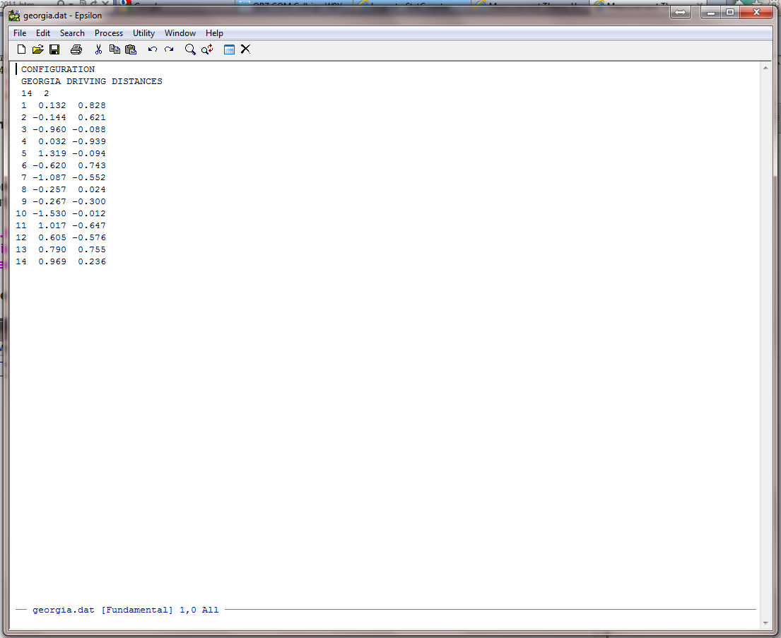
We want to save the original file so we are going to write a copy of georgia.dat to disk and we will call it gacoords.dat. Type the command:
C-X C-W -- This means Hold the Control key down and type X then hold the Control key down and type W" -- the Write File Command in Epsilon
You will see:

Now type the file name gacoords.dat:
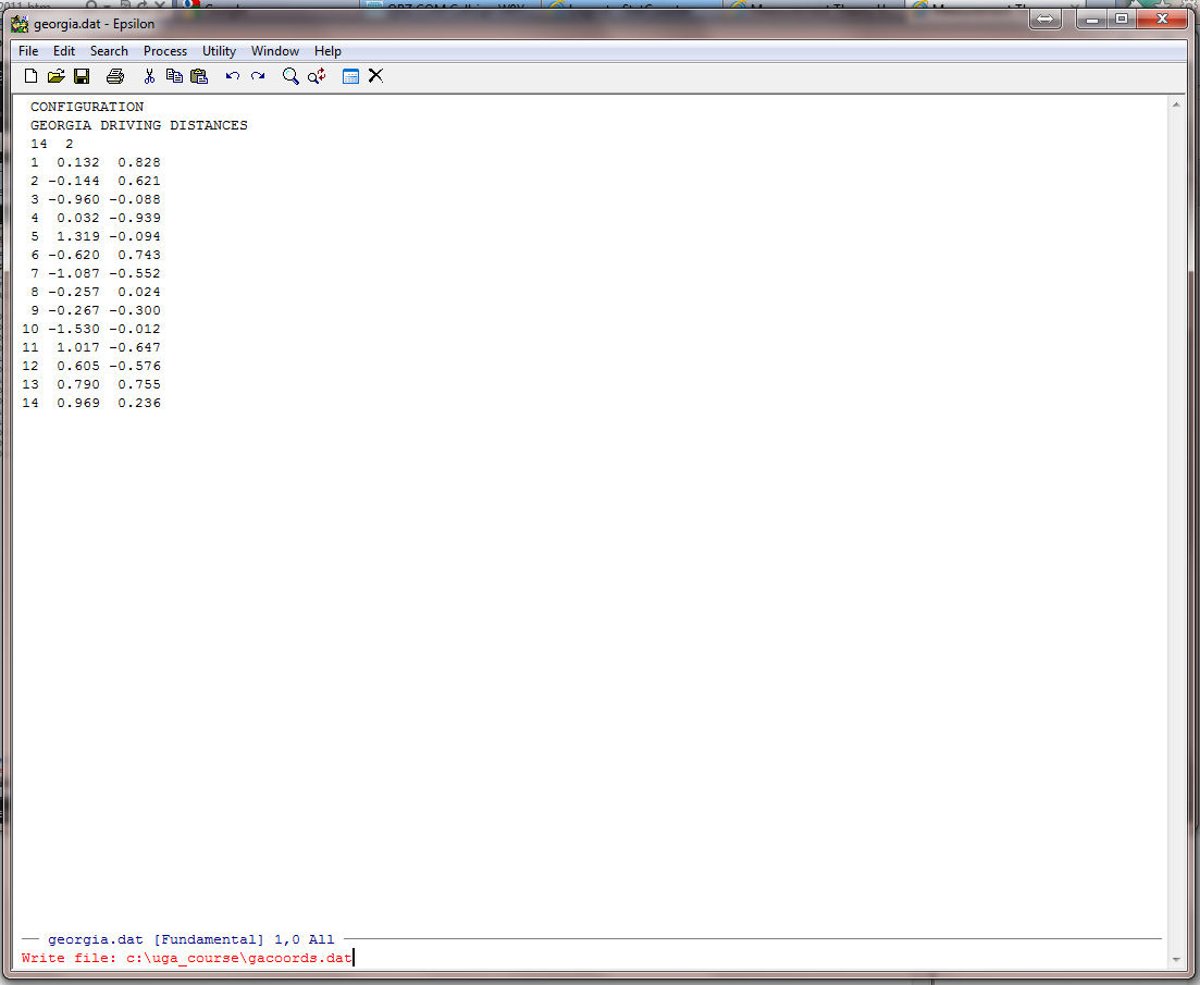
Now, just hit the Enter key and you should see:
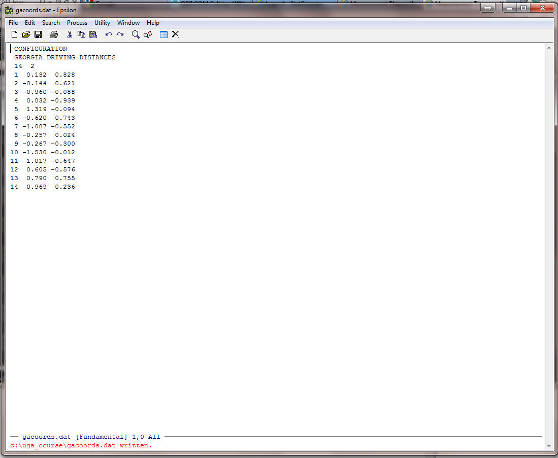
Now Type
C-X 2 -- This means "Hold the Control key down and type X and then type 2" (The Split Window Command in Epsilon)
You should see the following:

Note that your cursor will be in the bottom screen. Now we want to place georgia.txt in the bottom screen. To do this, use the command:
C-X C-F -- This means "Hold the Control key down and type X then hold the Control key down and type F" -- (The Find File Command in Epsilon)
You will see:

Now type georgia.txt:

Now, just hit the Enter key and you should have the two files in the split window:

Before continuing with the problem, you will sometimes want to find a file but you have forgotten the name. Suppose, however, you know what directory it is in. In the above, instead of typing georgia.txt at the end of the path statement, try simply hitting the Enter key. You will see:
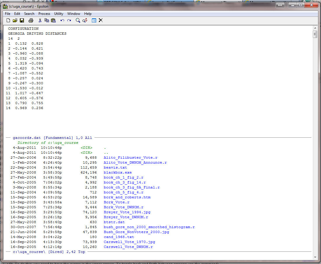
Epsilon lists all the files in the directory and the cursor will be positioned at the top. You can use the down and up arrow keys to move up and down the file list. Position the cursor at the beginning of the file you want and hit the Spacebar. The file will appear in the bottom window just as above. To close the screen your cursor is in you can use the command:
C-X 0 -- This means "Hold the Control key down and type X then type 0 (zero not ohh)" (This is the Kill Window command in Epsilon).
To close all screens except the one your cursor is in, you can use the command:
C-X 1 -- This means "Hold the Control key down and type X then type 1" (This is the Display only this Window command in Epsilon).
What we are going to do next is write a macro that will take the names of the cities from the georgia.txt file and insert them into the coordinates embedded in gacoords.dat. Before we begin, use the C-X p command (Select a Window command in Epsilon) to go down into the lower screen and position the cursor so that it is in front of "Albany" (Move to Window command in Epsilon). The C-X UP and The C-X DOWN commands (see the Selecting Windows Commands In the Epsilon Manual) also move UP (the up arrow key) and DOWN (the down arrow key) windows. Return to the upper screen using the C-X p or C-X UPcommand. To begin the macro, type:
C-X ( -- This means "Control-X" then "(" Start keyboard macro in Epsilon).
You will see:
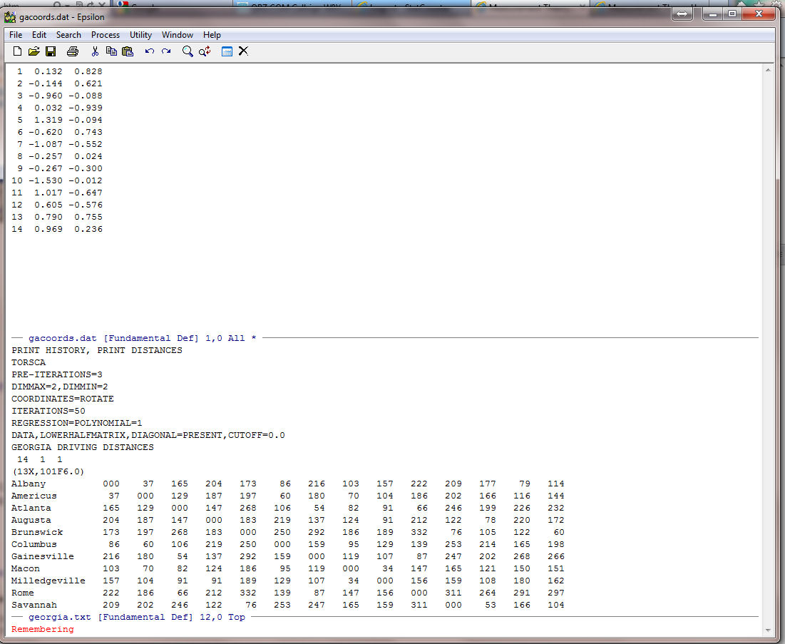
Note the Remembering at the bottom of the screen. Epsilon now records all the key-strokes that you enter until you give the command C-X ) (End keyboard macro in Epsilon). (Also note the asterisk "*" to the far right of the name line at the bottom of the top screen. This is a signal from Epsilon that the file has been altered and not saved. If you clicked on "File Save" that asterisk will not be there.) We will not need the numbers 1 to 32 that are before the two dimensional coordinates. So enter the command:
C-D C-D -- This means "Control-D" twice. (Delete Character in Epsilon). Note that this is exactly the same as hitting the Delete key twice. You should see:
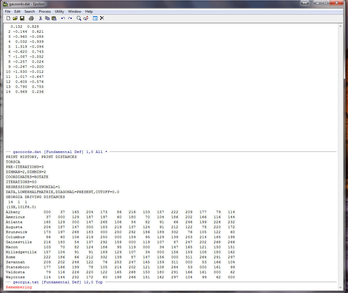
Now we are going down to the lower screen to pick up the names. To do this, first type:
C-X DOWN ( the Selecting Windows Commands In the Epsilon Manual)to go to the lower screen, then type
C-U (the argument command in Epsilon which is used to repeat keystrokes automatically). You will see:

Type 13 (the 4 disappears) and then C-F ( forward character in Epsilon). Your cursor will end up a few spaces to the right of the "000" (C-F is the same as Right-Arrow.) Now type:
Enter
And you should see:
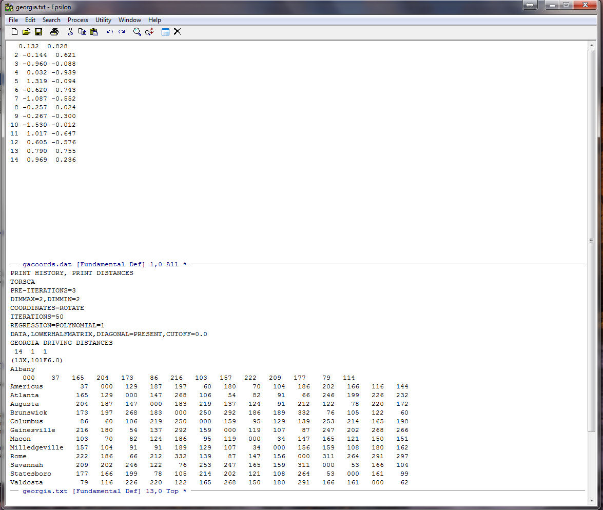
Now, enter the following commands one at a time:
C-P (up one line in Epsilon) This moves the cursor up one line so it is once again in front of "Albany"
C-K (kill line) Note that "Albany" disappears -- this places it in the "Kill Buffer"
C-Y (yank from Buffer) Viola, it disgorges it -- this "Yanks" the text from the buffer (the cursor will be at the end)
C-D (delete character) This re-assembles the original line.
C-A (go to the beginning of the line) This takes the cursor to the beginning of the line
C-N (move down one line) This positions the cursor at the beginning of the line below. We need to do this so that when the macro runs the first time it gets Americus, not Albany!!
C-X UP Go back up to the top screen
C-Y Yank Albany from the buffer
C-A Go to the beginning of the line
C-N Position the cursor at the beginning of the line below
C-X ) (end the keyboard macro) This ends the remembering and completes the macro.
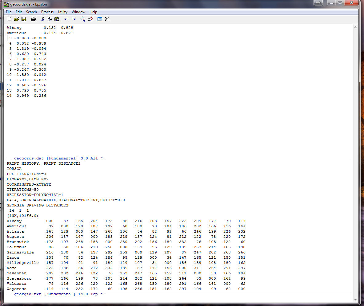
You should see:
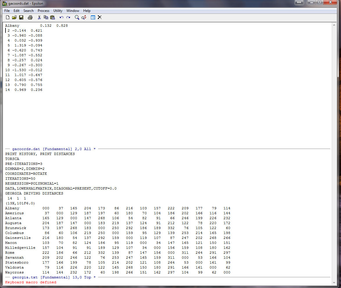
To execute the macro one time type:
C-X E (run keyboard macro one time) -- This means "hold the Control key down and type X then type E"
You should see:
Before executing the macro multiple times it is always good practice to check how many lines there are in the file so that you do not try to go beyond the end of the file (which can have some pretty nasty consequences). To do this type:
C-X L (count the number of lines in the file) -- This means "hold the Control key down and type X then type L"
You should see:

Epsilon tells you that there are 14 lines and the cursor is on line 3. We need to run the macro 12 times but lets execute it only 11 times just to be on the safe side (this is good practice!). To do this type:
C-U -- Control-U. You should see:
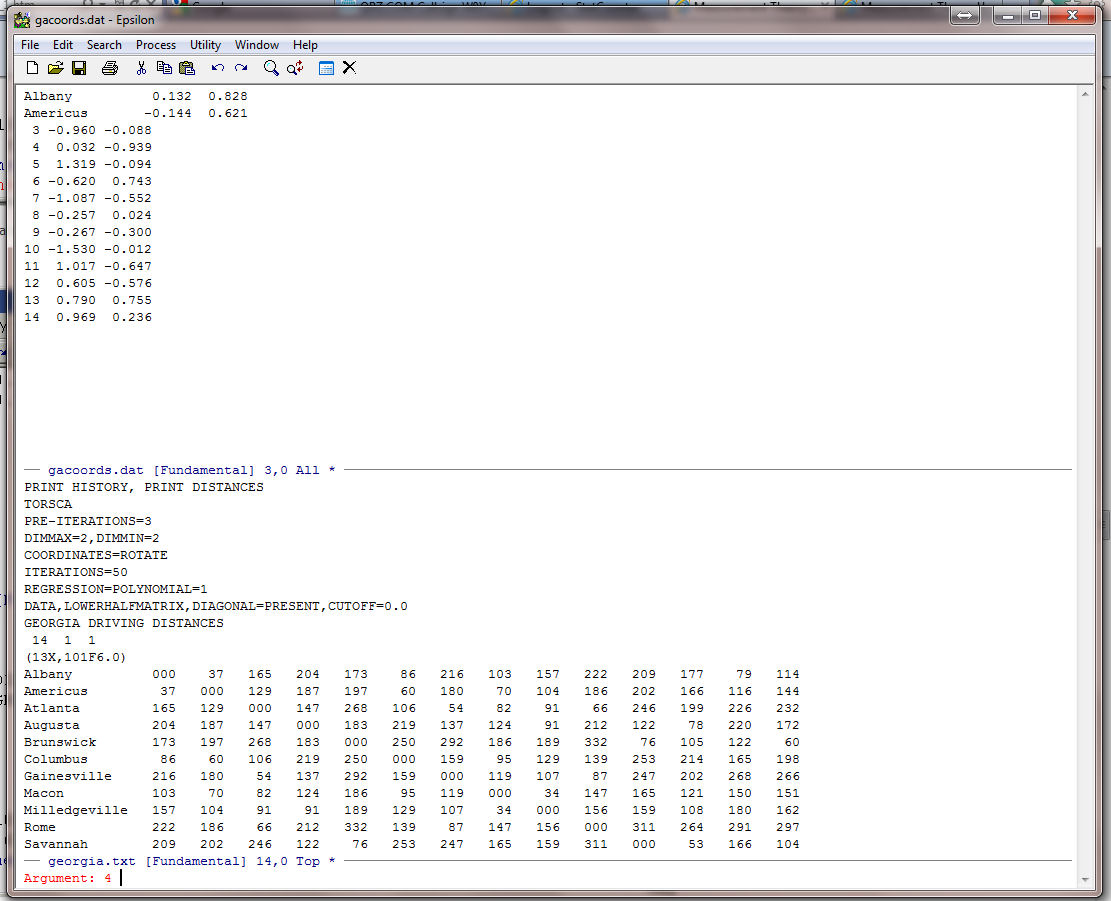
The C-U function will cause whatever command you enter next to be repeated. The "4" is a default. Simply type:
11 C-X E
You should see:
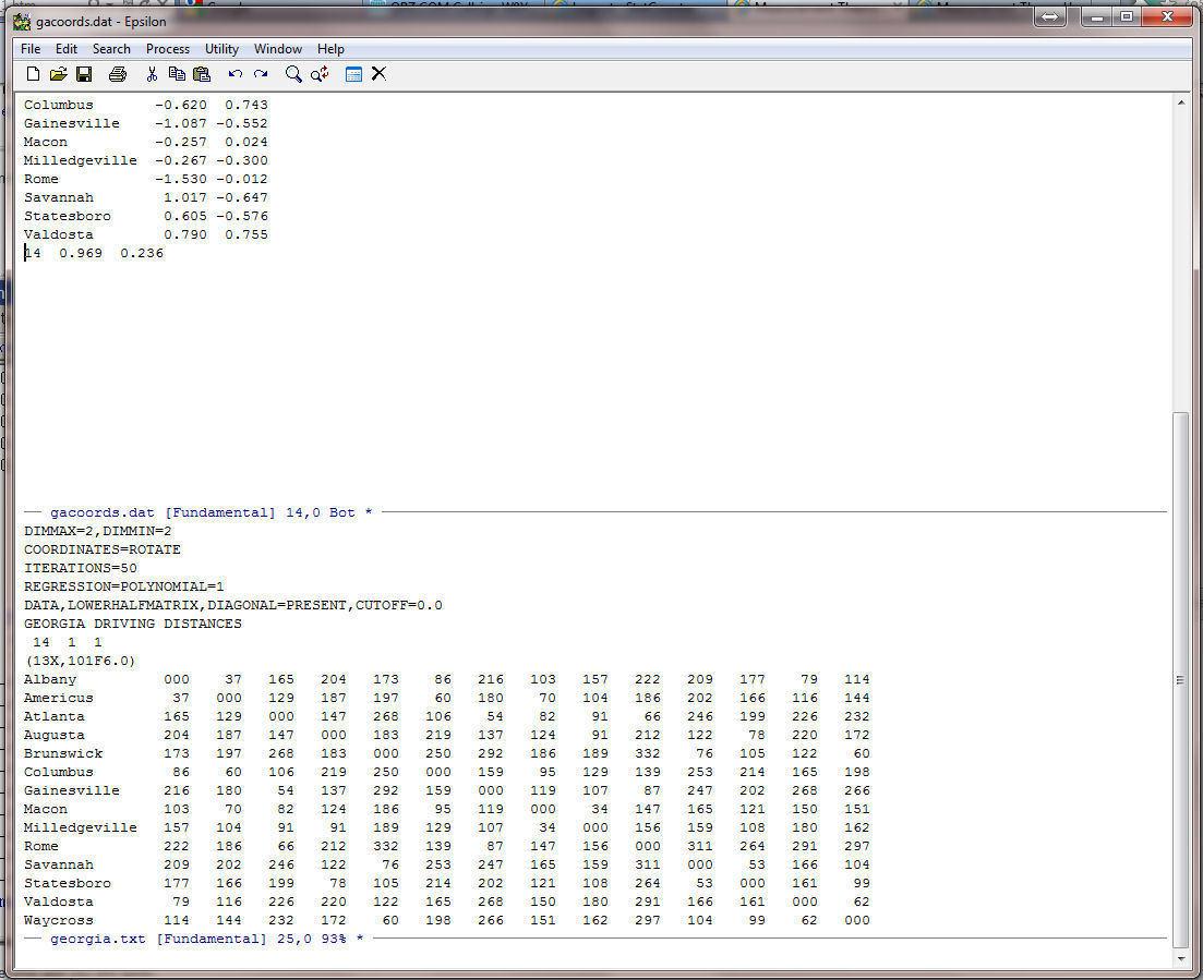
Now, simply execute the macro one more time and you are done:
C-X E
Your cursor should be right below Waycross. We no longer need georgia.txt so close the lower screen by typing (as described above):
C-X 1
Now save the file in the normal WINDOZE fashion by clicking the floppy token. You can also do this by typing the command:
C-X C-S (save file command)
Now, place the cursor back at the top of the file. You can do this by simply using the Page-Up but try the command:
ESC < -- This means "hit the Escape key then hit the < (less than) key.
To go to the bottom of the file use the command:
ESC >
(Note that the two commands are the same as:
ALT-< (go to the beginning of the file) -- Hold down the ALT key and type< (less than).
ALT-> (go to the end of the file) -- Hold down the ALT key and type> (greater than).)
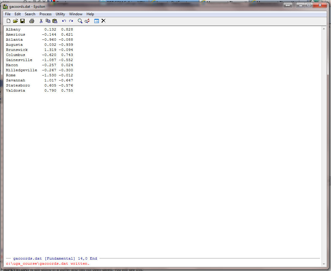
Now exit Epsilon. It will complain because georgia.txt is still sitting in a buffer and has not been saved. You will see this:

Click on "Exit" and it will flush the altered version of georgia.txt from its buffer and quit. If you look at georgia.txt on your disk drive it will be unaltered.
Now, start R
and enter the command: georgianames <- read.table("C:/uga_course/gacoords.dat",header=F,row.names=1)
This tells R to read in the file you just created. (Be sure to correctly type in the correct path statement!) The "header=F" tells R that we do not have labels for the columns and the "row.names=1" tells R that the first column are row labels. Now type:
georgianames
and you should see:
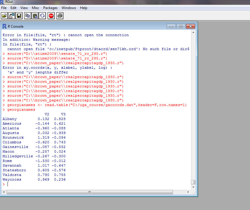
Note that R puts the default headers "V2" and "V3" above the coordinate columns! Now enter the commands:
attach(georgianames) -- This tells R that you want to work with the columns in "georgianames"
plot(V2,V3)
text(V2,V3,labels=row.names(georgianames),adj=0) -- This sticks the names into the plot!
- Turn in the above plot.
- Note that R has chopped off the names
on the right side. We can fix this by telling R
to change the scale of the axes. To do this enter the commands:
plot(V2,V3,xlim=c(-2,2),ylim=c(-2,2))
text(V2,V3,labels=row.names(georgianames),adj=0)
Turn in the above plot.
- Turn in the above plot.
- Continuing with the plotting exercise, download this R Program:
 Plot_Georgia.r -- Plot Program
#   The cross-hatch is used as a comment marker -- R ignores the line
# plot_georgia.r -- Does a graph of the 14 Cities using KYST output    Always put the name of the program at the top
#                       file gacoords.dat
#
# Albany         0.132  0.828    This is not necessary but I have no memory
# Americus      -0.144  0.621    so I always put in the file if its small so
# Atlanta       -0.960 -0.088    I do not forget what I am doing!
# Augusta        0.032 -0.939
# Brunswick      1.319 -0.094
# Columbus      -0.620  0.743
# Gainesville   -1.087 -0.552
# Macon         -0.257  0.024
# Milledgeville -0.267 -0.300
# Rome          -1.530 -0.012
# Savannah       1.017 -0.647
# Statesboro     0.605 -0.576
# Valdosta       0.790  0.755
# Waycross       0.969  0.236
#
#
#  Remove all objects just to be safe
#
rm(list=ls(all=TRUE))  This is not strictly necessary but I do not trust R
#
library(MASS)          This is a standard R library
#
#
#  %%%%%%%%%%%%%%%%%%%%%%%%%%%%%%%%%%%%%%%   The next set of commands read the file.
#  Read gacoords.dat                         This is admitedly clunky way of doing things
#  %%%%%%%%%%%%%%%%%%%%%%%%%%%%%%%%%%%%%%%   but it is bulletproof if you are careful.
#
rcx.file <- "c:/uga_course_homework_1/gacoords.dat"  Path to the File -- You need the quotes.
#
# Standard fields and their widths -- KYST output Legislators
#
rcx.fields <- c("name","dim1","dim2")   You need to name the columns.
rcx.fieldWidths <- c(13,7,7)            You need to give it the exact widths of the columns
#
# Input City Coordinates
#
T <- read.fwf(file=rcx.file,widths=rcx.fieldWidths,as.is=TRUE,col.names=rcx.fields) The Read Statement
dim(T)                   This Turns it into an R dataframe (which looks like a matrix)
#T <- as.matrix(T)       If you do not have any text in the dataset this command
#                        is handy because it makes your input data a true matrix and not a dataframe
names <- T[,1]
dimension1 <- T[,2]      These three commands just make life easier -- they are
dimension2 <- T[,3]      not necessary
#
#
nrow <- length(T[,1])    Here is how you can figure out the number of variables
ncol <- length(T[1,])    and the number of columns
#
#
#
#  This puts more white space
#    on the Right-Hand-Side Margin
#
par(mar=c(4.1,5.1,4.1,5.1))  This controls the margins on all 4 sides of the plot
#
#
plot(dimension1,dimension2,type="n",asp=1,  The "n" says no visible plot; asp=1 means
       main="",                             maintain the aspect ratio
       xlab="",
       ylab="",
       xlim=c(-2.0,2.0),ylim=c(-2.0,2.0))   These have to be the same for asp=1 to work
points(dimension1,dimension2,pch=16,col="red") Plot the Points
axis(1,font=2)                                 Horizontal axis in bold font
axis(2,font=2,cex=1.2)                         Vertical axis in bold font
# Main title
mtext("Georgia Cities From Driving Distances",side=3,line=1.00,cex=1.2,font=2)  Side 3 is the top
# x-axis title                                                                  line= controls position
mtext("This Seems to be Rotated",side=1,line=2.75,cex=1.2)
# y-axis title
mtext("Who the Heck Knows",side=2,line=2.5,cex=1.2)
#
# pos -- a position specifier for the text. Values of 1, 2, 3 and 4,
# respectively indicate positions below, to the left of, above and
# to the right of the specified coordinates
#
namepos <- rep(4,nrow)     This generates a nrow-length vector of 4's
#
#namepos[1] <- 4    # Albany
#namepos[2] <- 4    # Americus   I stuck in the City Names so
#namepos[3] <- 4    # Atlanta    You can control their positions
#namepos[4] <- 4    # Augusta
#namepos[5] <- 4    # Brunswick
#namepos[6] <- 4    # Columbus
#namepos[7] <- 4    # Gainesville
#namepos[8] <- 4    # Macon
#namepos[9] <- 4    # Milledgeville
#namepos[10] <- 4   # Rome
#namepos[11] <- 4   # Savannah
#namepos[12] <- 4   # Statesboro
#namepos[13] <- 4   # Valdosta
#namepos[14] <- 4   # Waycross
#
text(dimension1,dimension2,names,pos=namepos,offset=00.00,col="blue") This Plots the Names.
#                                       The offset= adjusts how far the name is from the point.
Run the program in R and you should get this:

- Produce a nice plot of the Cities by adjusting the positions of the names
in the namepos[] vector (just delete the "#" at the beginning of the line) and the
offset control. Turn in this plot.
- The Cities are clearly in the wrong orientation. Note that, because we are dealing with distances, the
configuration recovered by KYST is only going to be identified up to a choice of
origin and a rotation. In general, a rotation matrix in two dimensions is:

Where Q is the angle in radians. You can rotate the coordinates clockwise p/4 radians (45 degrees) with this code fragment:pi <- 3.141592653589793 pi4 <- pi/4 dimension1 <- cos(pi4)*T[,2] + sin(pi4)*(-1.0)*T[,3] dimension2 <- sin(pi4)*(-1.0)*T[,2] + cos(pi4)*(-1.0)*T[,3]
Note that I have flipped the sign on the second dimension in the formula above.
Use the above formula to rotate your configuration until it makes sense, properly label the X and Y axes by changing the labels in "mtext", and neatly arrange the city names. Turn in the Plot.
- Produce a nice plot of the Cities by adjusting the positions of the names
in the namepos[] vector (just delete the "#" at the beginning of the line) and the
offset control. Turn in this plot.
- Download the data file
 U. S. Map Driving Distance Data
and place it in the same folder with KYST.
The data file is reproduced below. It contains the lower half of a driving distance matrix computed between 10 U.S. cities -- Atlanta, Boise, Boston, Chicago, Cincinnati, Dallas, Denver, Los Angeles, Miami, and Washington, D.C..PRINT HISTORY, PRINT DISTANCES This Option Prints out Some Useful Intermediate Output DIMMAX=3, DIMMIN=1 TORSCA REGRESSION=POLYNOMIAL=1 METRIC MDS DATA,LOWERHALFMATRIX,DIAGONAL=PRESENT,CUTOFF=0.0 U.S. MAP EXAMPLE 10 1 1 (10f5.0) 0000 2340 0000 1084 2797 0000 715 1789 976 0000 481 2018 853 301 0000 826 1661 1868 936 988 0000 1519 891 2008 1017 1245 797 0000 2252 908 3130 2189 2292 1431 1189 0000 662 2974 1547 1386 1143 1394 2126 2885 0000 641 2480 443 696 498 1414 1707 2754 1096 0000 COMPUTE STOP
Run this data set through KYST and get the coordinates.
- Modify the Plot_Georgia.r program to make a plot of the 10 U.S. Cities. Turn in a
listing of the program and the two dimensional plot.
- Change REGRESSION=POLYNOMIAL=1 to
REGRESSION=ASCENDING and run it through KYST
(the "ascending"
tells KYST to do a Nonmetric MDS on
dissimilarity data). Compare the
Stress values for 1 to 3 dimensions with those obtained
above and compare the two dimensional plot obtained with this option to that in part (a).
- Modify the Plot_Georgia.r program to make a plot of the 10 U.S. Cities. Turn in a
listing of the program and the two dimensional plot.
- In this problem we are going to do a classic non-metric MDS on the Morse Code data.
Download data files:
 Morse Code Data Lower Half
 Morse Code Data Upper Half
and place it in the same folder with KYST. Here is what MORSEKYSTSL.DAT looks like:TORSCA PRE-ITERATIONS=3 DIMMAX=2,DIMMIN=2 PRINT HISTORY,PRINT DISTANCES COORDINATES=ROTATE ITERATIONS=50 REGRESSION=DESCENDING DATA,LOWERHALFMATRIX,DIAGONAL=PRESENT MORSE CODE DATA -- SIMILARITIES EXAMPLE 36 1 1 (1X,36F3.0) A 92 4 6 13 3 14 10 13 46 5 22 3 25 34 6 6 9 35 23 6 37 13 17 12 7 3 2 7 5 5 8 6 5 6 2 3 A B 5 84 37 31 5 28 17 21 5 19 34 40 6 10 12 22 25 16 18 2 18 34 8 84 30 42 12 17 14 40 32 74 43 17 4 4 B C 4 38 87 17 4 29 13 7 11 19 24 35 14 3 9 51 34 24 14 6 6 11 14 32 82 38 13 15 31 14 10 30 28 24 18 12 C D 8 62 17 88 7 23 40 36 9 13 81 56 8 7 9 27 9 45 29 6 17 20 27 40 15 33 3 9 6 11 9 19 8 10 5 6 D E 6 13 14 6 97 2 4 4 17 1 5 6 4 4 5 1 5 10 7 67 3 3 2 5 6 5 4 3 5 3 5 2 4 2 3 3 E F 4 51 33 19 2 90 10 29 5 33 16 50 7 6 10 42 12 35 14 2 21 27 25 19 27 13 8 16 47 25 26 24 21 5 5 5 F G 9 18 27 38 1 14 90 6 5 22 33 16 14 13 62 52 23 21 5 3 15 14 32 21 23 39 15 14 5 10 4 10 17 23 20 11 G H 3 45 23 25 9 32 8 87 10 10 9 29 5 8 8 14 8 17 37 4 36 59 9 33 14 11 3 9 15 43 70 35 17 4 3 3 H I 64 7 7 13 10 8 6 12 93 3 5 16 13 30 7 3 5 19 35 16 10 5 8 2 5 7 2 5 8 9 6 8 5 2 4 5 I J 7 9 38 9 2 24 18 5 4 85 22 31 8 3 21 63 47 11 2 7 9 9 9 22 32 28 67 66 33 15 7 11 28 29 26 23 J K 5 24 38 73 1 17 25 11 5 27 91 33 10 12 31 14 31 22 2 2 23 17 33 63 16 18 5 9 17 8 8 18 14 13 5 6 K L 2 69 43 45 10 24 12 26 9 30 27 86 6 2 9 37 36 28 12 5 16 19 20 31 25 59 12 13 17 15 26 29 36 16 7 3 L M 24 12 5 14 7 17 29 8 8 11 23 8 96 62 11 10 15 20 7 9 13 4 21 9 18 8 5 7 6 6 5 7 11 7 10 4 M N 31 4 13 30 8 12 10 16 13 3 16 8 59 93 5 9 5 28 12 10 16 4 12 4 16 11 5 2 3 4 4 6 2 2 10 2 N O 7 7 20 6 5 9 76 7 2 39 26 10 4 8 86 37 35 10 3 4 11 14 25 35 27 27 19 17 7 7 6 18 14 11 20 12 O P 5 22 33 12 5 36 22 12 3 78 14 46 5 6 21 83 43 23 9 4 12 19 19 19 41 30 34 44 24 11 15 17 24 23 25 13 P Q 8 20 38 11 4 15 10 5 2 27 23 26 7 6 22 51 91 11 2 3 6 14 12 37 50 63 34 32 17 12 9 27 40 58 37 24 Q R 13 14 16 23 5 34 26 15 7 12 21 33 14 12 12 29 8 87 16 2 23 23 62 14 12 13 7 10 13 4 7 12 7 9 1 2 R S 17 24 5 30 11 26 5 59 16 3 13 10 5 17 6 6 3 18 96 9 56 24 12 10 6 7 8 2 2 15 28 9 5 5 5 2 S T 13 10 1 5 46 3 6 6 14 6 14 7 6 5 6 11 4 4 7 96 8 5 4 2 2 6 5 5 3 3 3 8 7 6 14 6 T U 14 29 12 32 4 32 11 34 21 7 44 32 11 13 6 20 12 40 51 6 93 57 34 17 9 11 6 6 16 34 10 9 9 7 4 3 U V 5 17 24 16 9 29 6 39 5 11 26 43 4 1 9 17 10 17 11 6 32 92 17 57 35 10 10 14 28 79 44 36 25 10 1 5 V W 9 21 30 22 9 36 25 15 4 25 29 18 15 6 26 20 25 61 12 4 19 20 86 22 25 22 10 22 19 16 5 9 11 6 3 7 W X 7 64 45 19 3 28 11 6 1 35 50 42 10 8 24 32 61 10 12 3 12 17 21 91 48 26 12 20 24 27 16 57 29 16 17 6 X Y 9 23 62 15 4 26 22 9 1 30 12 14 5 6 14 30 52 5 7 4 6 13 21 44 86 23 26 44 40 15 11 26 22 33 23 16 Y Z 3 46 45 18 2 22 17 10 7 23 21 51 11 2 15 59 72 14 4 3 9 11 12 36 42 87 16 21 27 9 10 25 66 47 15 15 Z 1 2 5 10 3 3 5 13 4 2 29 5 14 9 7 14 30 28 9 4 2 3 12 14 17 19 22 84 63 13 8 10 8 19 32 57 55 1 2 7 14 22 5 4 20 13 3 25 26 9 14 2 3 17 37 28 6 5 3 6 10 11 17 30 13 62 89 54 20 5 14 20 21 16 11 2 3 3 8 21 5 4 32 6 12 2 23 6 13 5 2 5 37 19 9 7 6 4 16 6 22 25 12 18 64 86 31 23 41 16 17 8 10 3 4 6 19 19 12 8 25 14 16 7 21 13 19 3 3 2 17 29 11 9 3 17 55 8 37 24 3 5 26 44 89 42 44 32 10 3 3 4 5 8 45 15 14 2 45 4 67 7 14 4 41 2 0 4 13 7 9 27 2 14 45 7 45 10 10 14 10 30 69 90 42 24 10 6 5 5 6 7 80 30 17 4 23 4 14 2 11 11 27 6 2 7 16 30 11 14 3 12 30 9 58 38 39 15 14 26 24 17 88 69 14 5 14 6 7 6 33 22 14 5 25 6 4 6 24 13 32 7 6 7 36 39 12 6 2 3 13 9 30 30 50 22 29 18 15 12 61 85 70 20 13 7 8 3 23 40 6 3 15 15 6 2 33 10 14 3 6 14 12 45 2 6 4 6 7 5 24 35 50 42 29 16 16 9 30 60 89 61 26 8 9 3 14 23 3 1 6 14 5 2 30 6 7 16 11 10 31 32 5 6 7 6 3 8 11 21 24 57 39 9 12 4 11 42 56 91 78 9 0 9 3 11 2 5 7 14 4 5 30 8 3 2 3 25 21 29 2 3 4 5 3 2 12 15 20 50 26 9 11 5 22 17 52 81 94 0 COMPUTE STOP
This is the famous morse code data. If you compare this file to MORSEKYSTSU.DAT they are exactly the same except the matrix is transposed.
- Run MORSEKYSTSL.DAT and MORSEKYSTSU.DAT through KYST (be sure to use
unique output file names) in 1 to 3 dimensions. To do this change:
DIMMAX=2,DIMMIN=2 to
DIMMAX=3,DIMMIN=1
using Epsilon. Report the Stress values for 1 to 3 dimensions for the two halves of the data.
- Make two-dimensional Plots for the two halves of the data (use Epsilon
to put the 26 letters and 10 integers before the corresponding coordinates). (You can modify the
Plot_Georgia.r program to do this.) Turn in the plots and the
R code. Do the plots look the same?
- Run MORSEKYSTSL.DAT and MORSEKYSTSU.DAT through KYST (be sure to use
unique output file names) in 1 to 3 dimensions. To do this change: