---

1. In this problem we are going to analyze the nations data with a more realistic Likelihood Function where we assume that the observed distances have a log-normal distribution. We are also going to take a Bayesian approach and state prior distributions for all of the parameters of our model. Hence, rather than minimizing a squared-error loss function we are going to maximize the log-likelihood of a posterior distribution.
   
   We assume that our observed distances have the log normal distribution:
   
   
   Which produces the Likelihood Function:
   
   
   Our prior distributions for the coordinates and the variance are:
   
   
   And the log of our Posterior Distribution is:
   
   
   We are going to use a version of metric_mds_nations_ussr_usa.r which we used in Homeword 5, Question 3 to find the coordinates and the variance term that maximizes the log-liklihood of the posterior distribution.
   
   Download the R program:
   
   metric_mds_nations_log_normal_2.r -- Program to optimize the Log-Normal Bayesian Model for the Nations data.
   
   Here is the function that computes the log-likelihood:

   
   fr <- function(zzz){
   #
   xx[1:18] <- zzz[1:18]
   xx[21] <- zzz[19]
   xx[19:20] <- 0.0
   xx[22] <- 0.0
   xx[23:24] <- zzz[20:21]
   sigmasq <- zzz[22]          We have an additional parameter -- the variance term of the log-normal
   kappasq <- 100.0            The variance term of the Coordinate priors
   sumzsquare <- sum(zzz[1:21]**2) Sum of the squared coordinates
   #
   i <- 1
   sse <- 0.0
   while (i <= np) {
     ii <- 1
     while (ii <= i) {
      j <- 1
      dist_i_ii <- 0.0
      while (j <= ndim) {
   #
   #  Calculate distance between points
   #
          dist_i_ii <- dist_i_ii + (xx[ndim*(i-1)+j]-xx[ndim*(ii-1)+j])*(xx[ndim*(i-1)+j]-xx[ndim*(ii-1)+j])
          j <- j + 1
          }            Note that this is the sum of squared differences of the logs
         if (i != ii)sse <- sse + (log(sqrt(TT[i,ii])) - log(sqrt(dist_i_ii)))**2
         ii <- ii + 1
        }
      i <- i + 1
      }   Here we have to include the variance term and the logs of the priors
     sse <- (((np*(np-1))/2.0)/2.0)*log(sigmasq)+(1/(2*sigmasq))*sse+(1/(2*kappasq))*sumzsquare
   return(sse)  Note that above we have multiplied the log-likelihood by -1 so that the optimizers will find a minimum
   }

   The number of parameters is equal to 22 (nparam=22) now and further down in the problem before the optimizers are called zzz[22] is initialized to 0.2.
   
   
   1. Run the program and turn in a NEATLY FORMATTED plot of the nations.
      
      
   2. Report xfit and rfit and a NEATLY FORMATTED listing of results.
      
      
   3. Add the code to produce a graph of the eigenvalues of the Hessian matrix. Turn in NEATLY FORMATTED versions of this plot with appropriate labeling.
      
      
2. In problem (1) we used General Purpose Optimization Routine -- optim -- in R to find a mode that is, hopefully, the global minimum of our posterior distribution. Now we are going to use WINBUGS to analyze our posterior distribution. (If you need a refresher inWINBUGS go to my Bayes by the Beach Page and go through the Gary King Data Example. It has detailed screen shots of how to use WinBUGS.) Specifically, we are going to use RtoWinBUGS (Download) (Documentation). Download the R program and the text files it uses:
   
   nations_RtoWinbugs.r -- Program to run the Log-Normal Bayesian Model on the Nations data.
   
   nations_bayes_model.txt -- Model used by WINBUGS
   nations.txt -- Nations Data used by WINBUGS
   
   
   Here is the R Program:

   #
   #
   # Wish 1971 nations similarities data
   # Title: Perceived similarity of nations
   #
   # Description: Wish (1971) asked 18 students to rate the global
   # similarity of different pairs of nations such as 'France and China' on
   # a 9-point rating scale ranging from `1=very different' to `9=very
   # similar'. The table shows the mean similarity ratings. 
   #
   # Brazil      9.00 4.83 5.28 3.44 4.72 4.50 3.83 3.50 2.39 3.06 5.39 3.17
   # Congo       4.83 9.00 4.56 5.00 4.00 4.83 3.33 3.39 4.00 3.39 2.39 3.50
   # Cuba        5.28 4.56 9.00 5.17 4.11 4.00 3.61 2.94 5.50 5.44 3.17 5.11
   # Egypt       3.44 5.00 5.17 9.00 4.78 5.83 4.67 3.83 4.39 4.39 3.33 4.28
   # France      4.72 4.00 4.11 4.78 9.00 3.44 4.00 4.22 3.67 5.06 5.94 4.72
   # India       4.50 4.83 4.00 5.83 3.44 9.00 4.11 4.50 4.11 4.50 4.28 4.00
   # Israel      3.83 3.33 3.61 4.67 4.00 4.11 9.00 4.83 3.00 4.17 5.94 4.44
   # Japan       3.50 3.39 2.94 3.83 4.22 4.50 4.83 9.00 4.17 4.61 6.06 4.28
   # China       2.39 4.00 5.50 4.39 3.67 4.11 3.00 4.17 9.00 5.72 2.56 5.06
   # USSR        3.06 3.39 5.44 4.39 5.06 4.50 4.17 4.61 5.72 9.00 5.00 6.67
   # USA         5.39 2.39 3.17 3.33 5.94 4.28 5.94 6.06 2.56 5.00 9.00 3.56
   # Yugoslavia  3.17 3.50 5.11 4.28 4.72 4.00 4.44 4.28 5.06 6.67 3.56 9.00
   #
   rm(list=ls(all=TRUE))
   #
   library(arm)      The arm library calls a series of other libraries including RtoWinBUGS
   setwd("C:/uga_course_homework_6")
   #
   #
   #  Read Nations Similarities Data
   #
   T <- matrix(scan("C:/uga_course_homework_6/nations.txt",0),ncol=12,byrow=TRUE)
   TT <- 9-T   Note the Subtraction -- We need Distances/Dissimilarities, not Similarities
   dim(TT)
   #
   nrow <- length(TT[,1])
   #ncol <- length(TT[1,])
                             Setup for passing our distances as a List
   V <- cbind(TT[,1],TT[,2],TT[,3],TT[,4],TT[,5],TT[,6],TT[,7],TT[,8],TT[,9],TT[,10],TT[,11],TT[,12])
   
   N = nrow
   K = ncol(V)
   
   data.data = list(dstar=V) Our distance data as a list
                             initializing our variables
   data.inits = function() {list(x=runif(2*K,-2,2), tau=runif(1,0,10))}
   
                             Variables we want analyzed in the WinBUGS Script
   data.parameters = c("x","tau","sumllh2")
                             Here is the call to WinBUGS14
                             Documentation for the bugs call
   wide.sim = bugs(data.data, data.inits, data.parameters,bugs.directory="c:/WinBUGS14/",model.file="nations_bayes_model.txt", n.chains=4, n.thin=1, n.burnin=15000,n.iter=100000, debug=TRUE,digits=5)
   #wide.sim = bugs(data.data, inits=NULL, data.parameters,bugs.directory="c:/WinBUGS14/",model.file="nations_bayes_model.txt", n.chains=4, n.thin=1, n.burnin=15000,n.iter=40000, debug=TRUE)
   
   detach(data)

   Here is the Model Analyzed by WINBUGS -- nations_bayes_model.txt:

   
   #
   #  MDS Model for Nations Data
   #
   model{
   #
   #  Fix USSR       Constraints on the USSR and USA
   #
            x[10,1] <- 0.000
   	 x[10,2] <- 0.000
   #
   #  Fix USA 2nd Dimension
   #
            x[11,2] <- 0.000
   #
   for (i in 1:11){           This Loop Computes the Log-Likelihood
             llh[i,i] <- 0.0
   	  for (j in i+1:12){
   #
   #
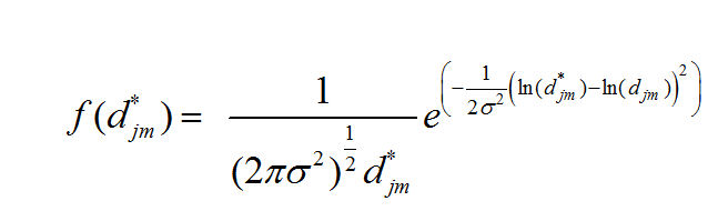
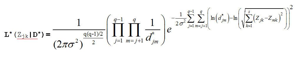
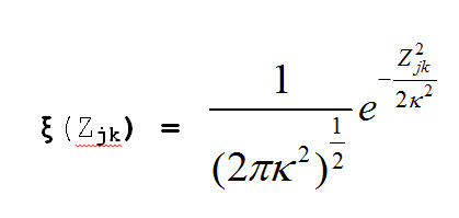
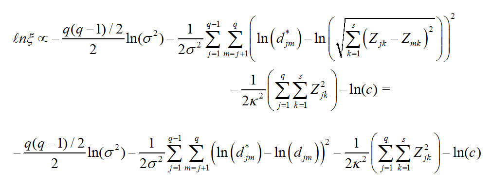
   	         dstar[i,j] ~ dlnorm(mu[i,j],tau)
                    mu[i,j] <- log(sqrt((x[i,1]-x[j,1])*(x[i,1]-x[j,1])+(x[i,2]-x[j,2])*(x[i,2]-x[j,2])))
                    llh[i,j] <- (log(dstar[i,j])-mu[i,j])*(log(dstar[i,j])-mu[i,j])
                    llh[j,i] <- (log(dstar[i,j])-mu[i,j])*(log(dstar[i,j])-mu[i,j])
   	     }
   	  }
   #
   #  Borrowed From Simon Jackman  Simple Trick to Keep track of the log-likelihood
   #
             llh[12,12] <- 0.0
      sumllh2 <- sum(llh[,])
   #
      
     ## priors   Priors on the Parameters
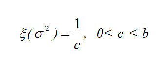
     tau ~ dgamma(.1,.1)
   #
     for(l in 1:2){x[1,l] ~ dnorm(0.0, 0.01)}
     x[2,1] ~ dnorm(0.0,0.01)
     for(l in 1:2){
         for(k in 3:6) {x[k,l] ~ dnorm(0.0, 0.01)}
     }
     x[7,2] ~ dnorm(0.0,0.01)
     x[8,1] ~ dnorm(0.0,0.01)
     x[9,2] ~ dnorm(0.0,0.01)
     x[11,1] ~ dnorm(0.0,0.01)
     for(l in 1:2){x[12,l] ~ dnorm(0.0, 0.01)}
   #
   #  Kludge to fix rotation -- set 1st and 2nd dimension coordinates of
   #          4 Nations to fix the sign flips
   #
      x[2,2] ~ dnorm(0.0,0.01)I(0,) 2nd Dimension Congo > 0
      x[7,1] ~ dnorm(0.0,0.01)I(0,) 1st Dimension Israel > 0
      x[8,2] ~ dnorm(0.0,0.01)I(,0) 2nd Dimension Japan < 0
      x[9,1] ~ dnorm(0.0,0.01)I(,0) 1st Dimension China < 0
   }

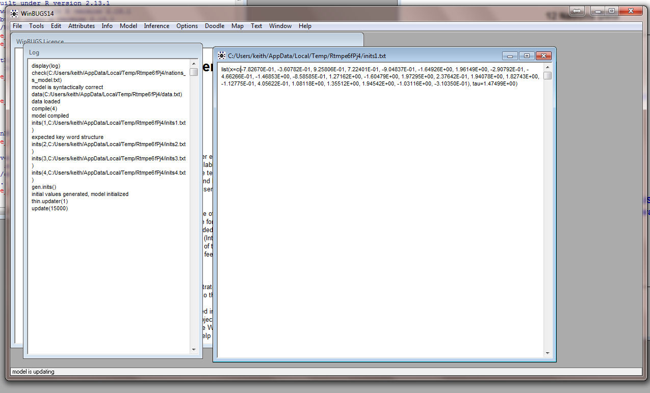
   When you load nations_RtoWinbugs.r into R it starts WinBUGS. You can watch WINBUGS in operation by bringing it to the front and it should look something like this:
   
   
   
   This is what it looks like when it is finished. Note the Path Statement!!
   
   
   
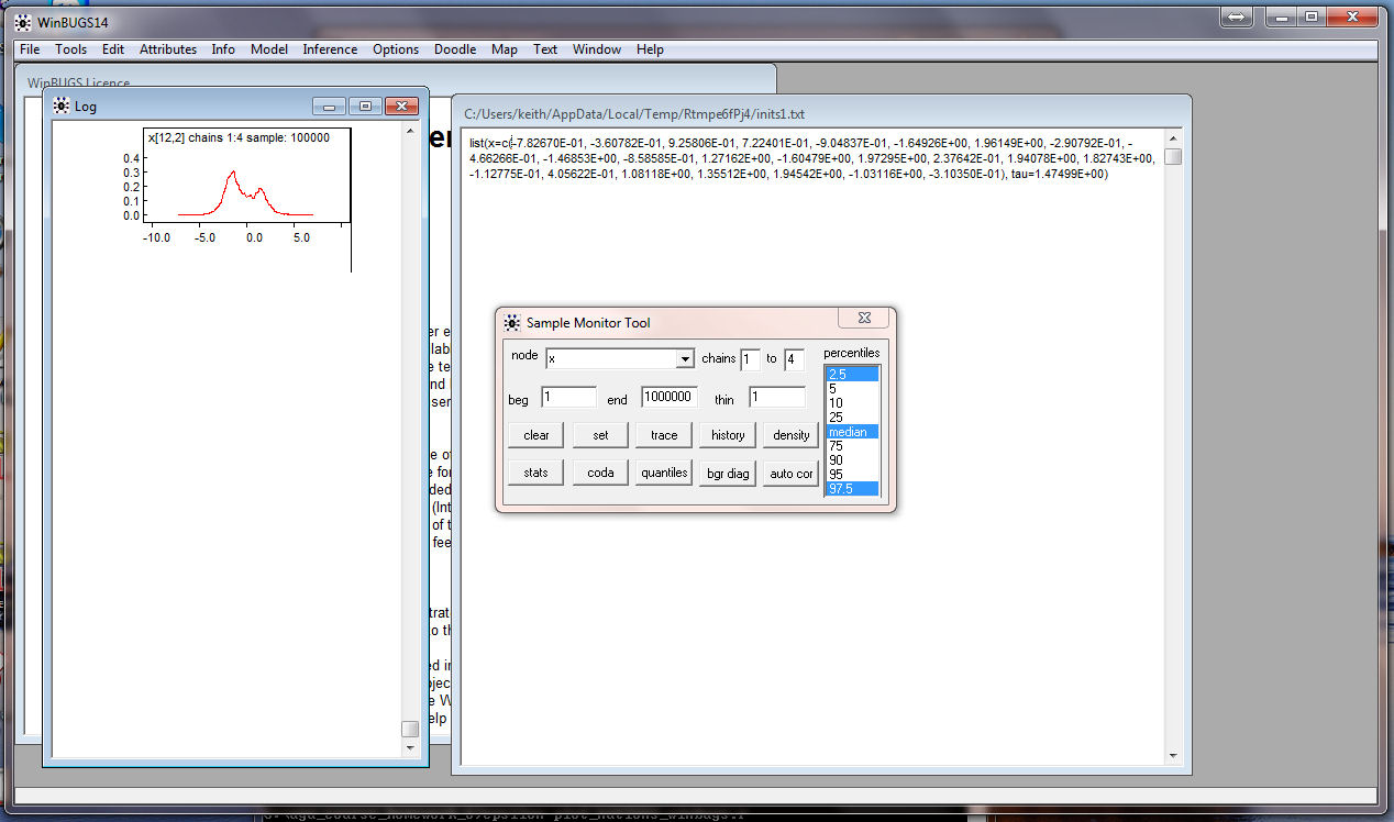
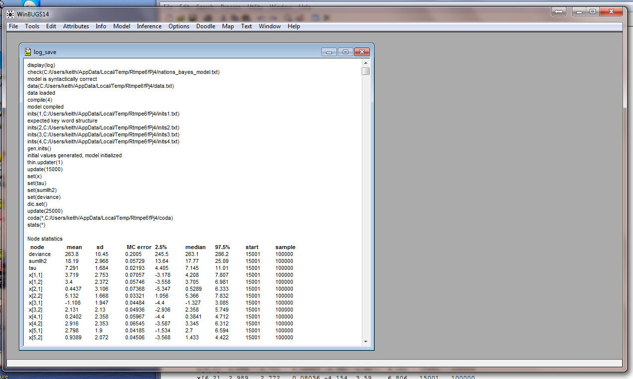
   WinBUGS is still running so you can get more information about the estimation than is provided in the default. In particular, we want to see the Density for each of the variables. Under Inference select Samples from the drop-down menu and you get the Sample Monitor Tool
   
   
   
   Put x in the node window and click on density and all the densities for the coordinates appear:
   
   
   
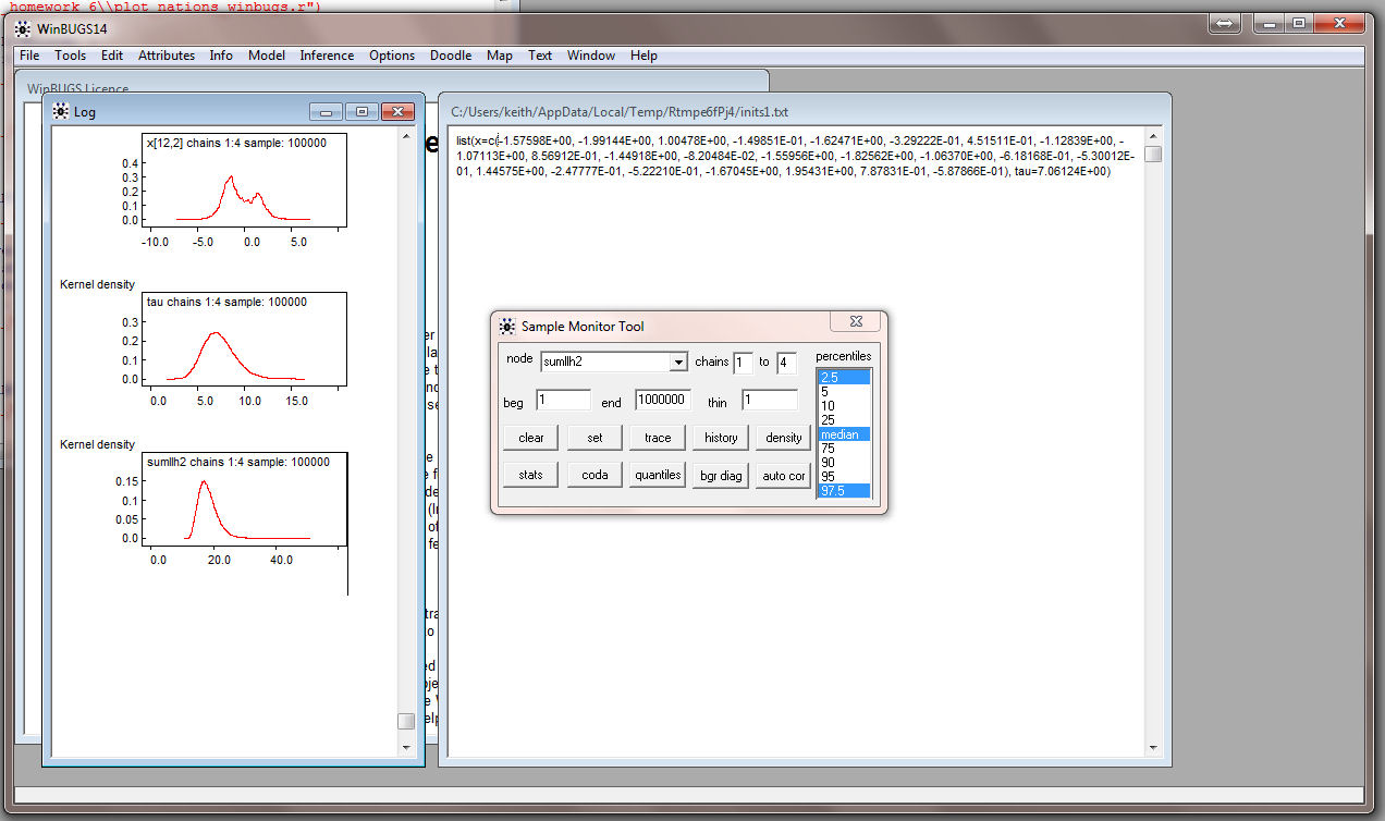
   Similarly, get the density for tau:
   
   
   
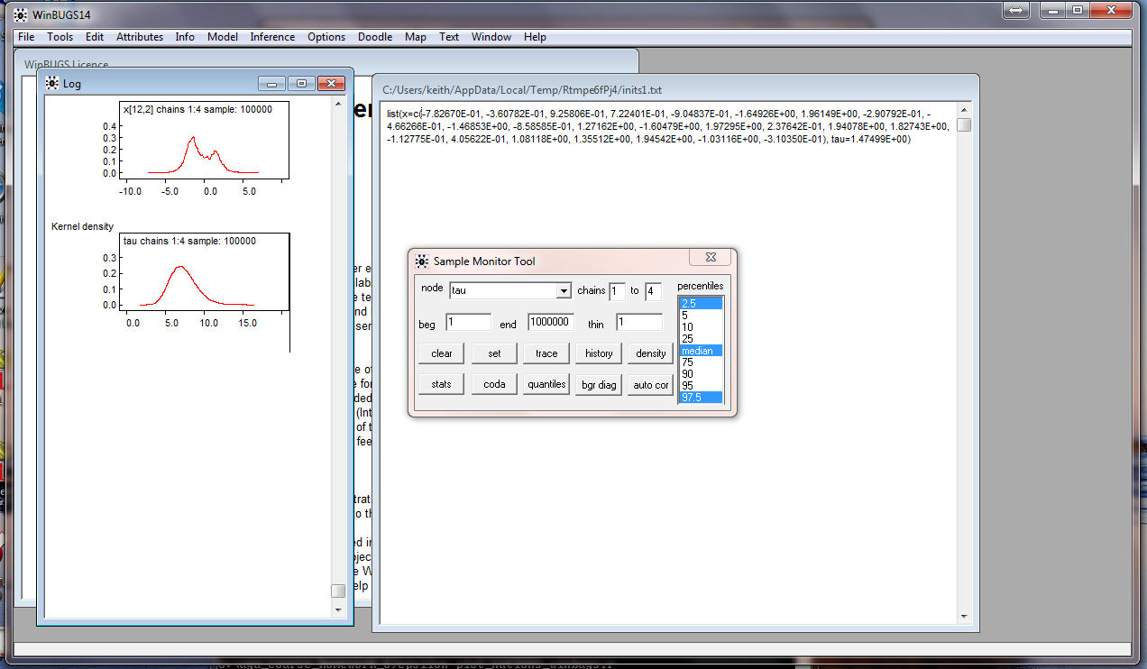
   and the density for the log-likelihood (sumllh2):
   
   
   
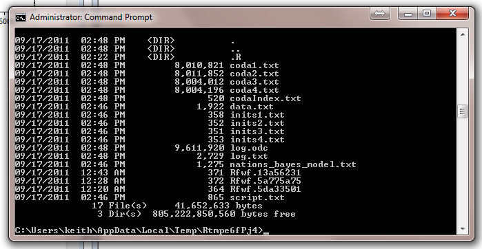
   Be sure to have a Command Prompt running and go to the directory where WinBUGS has written the output files. This is what it should look like:
   
   
   
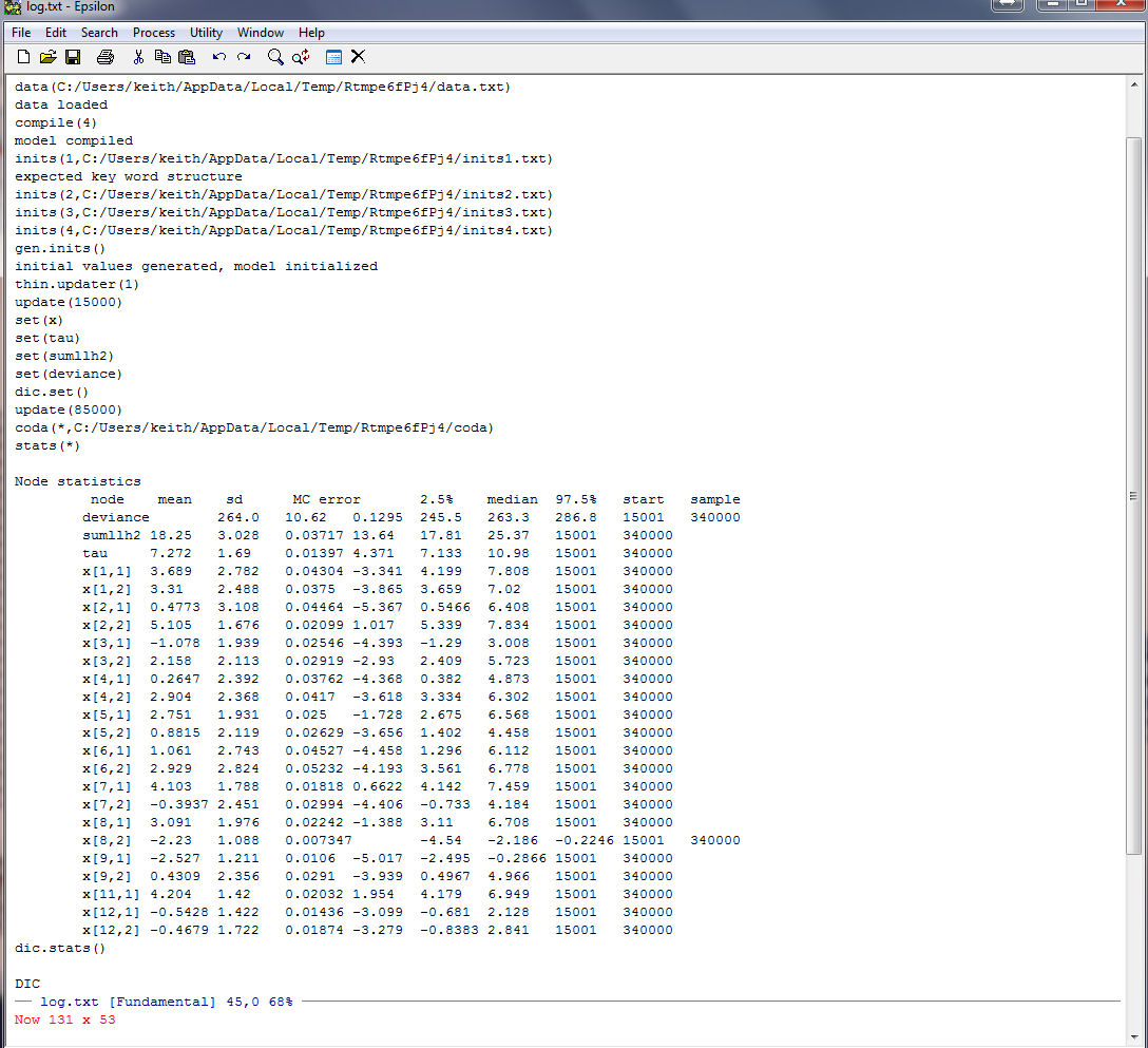
   Use Epsilon to bring up log.txt (we will use this below):
   
   
   
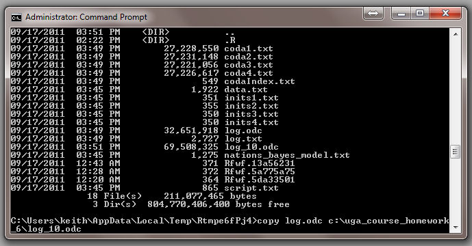
   Since we have the densities in the output log file copy log.odc over to your directory but rename it something like log_10.odc:
   
   
   
   Always have a spare copy of WinBUGS running. You can now open log_10.odc in WinBUGS:
   
   
   
   And it should look like this:
   
   
   
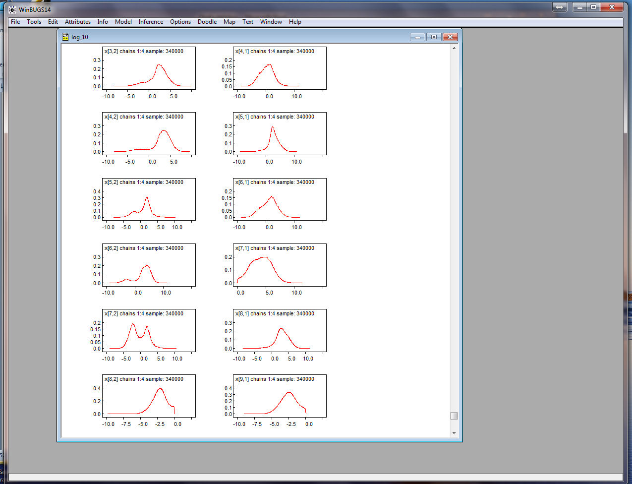
   You can copy the Density plots and paste them into MICROSHAFT WORD (be sure to use the Paste Special option):
   
   
   
   Below are screen shots of the Densities for all of the parameters:
   
   
   
   Note that some of the coordinates have two modes! Also note that you can pick out those coordinates that have been constrained!
   
   
   
   
   
   Here are the mean coordinates from our WinBUGS run. Note that the standard errors are not real great but OK.
   
   
   
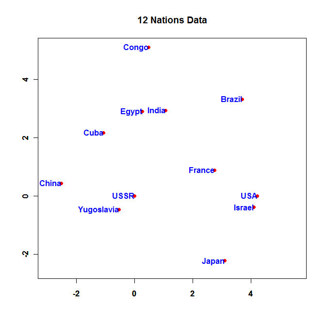
   And here is a plot of the Nations from WinBUGS:
   
   
   
   
   1. Run the R program above and put the Node Statistics Table into WORD NEATLY FORMATTED! Paste in the Densities for Deviance, sumllh2, and tau. Show every multi-mode coordinate density and identify the country.
      
      
   2. Neatly graph the mean coordinates from your WinBUGS run and turn in the R code you used to make the plot.
      
      
3. Let A be the matrix of Nation coordinates from question (1) and B be the matrix of Nation coordinates from question (2). Using the same method as Question 4 of Homework 5 solve for the orthogonal procrustes rotation matrix, T, for B.
   
   
   1. Solve for T and turn in a neatly formatted listing of T. Compute the Pearson r-squares between the corresponding columns of A and B before and after rotating B.
      
      
   2. Do a two panel graph with the two plots side-by-side -- A on the left and B on the right.