In question (1) of Homework 9 we used General Purpose Optimization Routine --
optim -- in R to find a
mode that is, hopefully, the global minimum of our
posterior distribution. Now we are
going to use
JAGS to analyze
our posterior distribution.
Specifically, we are going to use
rjags
(Download).
Download the R
program and the text files it uses:
 JAGS_mds_nations.r
-- Program to run the Log-Normal Bayesian Model on the Nations
data.
Here is the R Program:#
#
# Wish 1971 nations similarities data
# Title: Perceived similarity of nations
#
# Description: Wish (1971) asked 18 students to rate the global
# similarity of different pairs of nations such as 'France and China' on
# a 9-point rating scale ranging from `1=very different' to `9=very
# similar'. The table shows the mean similarity ratings.
#
# Brazil 9.00 4.83 5.28 3.44 4.72 4.50 3.83 3.50 2.39 3.06 5.39 3.17
# Congo 4.83 9.00 4.56 5.00 4.00 4.83 3.33 3.39 4.00 3.39 2.39 3.50
# Cuba 5.28 4.56 9.00 5.17 4.11 4.00 3.61 2.94 5.50 5.44 3.17 5.11
# Egypt 3.44 5.00 5.17 9.00 4.78 5.83 4.67 3.83 4.39 4.39 3.33 4.28
# France 4.72 4.00 4.11 4.78 9.00 3.44 4.00 4.22 3.67 5.06 5.94 4.72
# India 4.50 4.83 4.00 5.83 3.44 9.00 4.11 4.50 4.11 4.50 4.28 4.00
# Israel 3.83 3.33 3.61 4.67 4.00 4.11 9.00 4.83 3.00 4.17 5.94 4.44
# Japan 3.50 3.39 2.94 3.83 4.22 4.50 4.83 9.00 4.17 4.61 6.06 4.28
# China 2.39 4.00 5.50 4.39 3.67 4.11 3.00 4.17 9.00 5.72 2.56 5.06
# USSR 3.06 3.39 5.44 4.39 5.06 4.50 4.17 4.61 5.72 9.00 5.00 6.67
# USA 5.39 2.39 3.17 3.33 5.94 4.28 5.94 6.06 2.56 5.00 9.00 3.56
# Yugoslavia 3.17 3.50 5.11 4.28 4.72 4.00 4.44 4.28 5.06 6.67 3.56 9.00
#
rm(list=ls(all=TRUE))
#
library(rjags)
#
load(url("https://legacy.voteview.com/k7ftp/wf1/nations.Rda"))
#
d <- 9 - nations
N <- nrow(d)
K <- ncol(d)
inits <- function() {
z <- matrix(runif(2*K, -5, 5), nrow=K, ncol=2)
z[10,1] <- z[10,2] <- z[11,2] <- NA
z[2,2] <- abs(z[2,2])
z[7,1] <- abs(z[7,1])
z[8,2] <- -abs(z[8,2])
z[9,1] <- -abs(z[9,1])
list("z"= z, "tau"=runif(1,0,10))}
#
jags <- jags.model(
url("https://legacy.voteview.com/k7ftp/wf1/JAGS_mds_model.bug"),
data = list('N' = N, 'dstar' = d), inits = inits,
n.chains = 2, n.adapt = 10000)
#
update(jags, n.iter = 30000)
#
z <- coda.samples(jags, 'z', 10000, thin = 10)
Here is the Model Analyzed by JAGS -- JAGS_mds_model.bug:
#
#  MDS Model for Nations Data
#
model{
#
# Fix USSR
#
        z[10,1] <- 0.000
        z[10,2] <- 0.000
#
#  Fix USA 2nd Dimension
#
        z[11,2] <- 0.000
#
for (i in 1:N-1){
	  for (j in i+1:N){
#
#
dstar[i,j] ~ dlnorm(mu[i,j],tau)
                 mu[i,j] <- log(sqrt((z[i,1]-z[j,1])*(z[i,1]-z[j,1])+(z[i,2]-z[j,2])*(z[i,2]-z[j,2])))
	     }
	  }
#
## priors
#
tau ~ dunif(0,10)
#
  for(l in 1:2){z[1,l] ~ dnorm(0.0, 0.01)}
  z[2,1] ~ dnorm(0.0,0.01)
  for(l in 1:2){
      for(k in 3:6) {z[k,l] ~ dnorm(0.0, 0.01)}
  }
  z[7,2] ~ dnorm(0.0,0.01)
  z[8,1] ~ dnorm(0.0,0.01)
  z[9,2] ~ dnorm(0.0,0.01)
  z[11,1] ~ dnorm(0.0,0.01)
  for(l in 1:2){z[12,l] ~ dnorm(0.0, 0.01)}
#
#  Kludge to fix rotation -- set 1st and 2nd dimension coordinates of
#          4 Nations to fix the sign flips

   z[2,2] ~ dnorm(0.0,0.01)I(0,)
   z[7,1] ~ dnorm(0.0,0.01)I(0,)
   z[8,2] ~ dnorm(0.0,0.01)I(,0)
   z[9,1] ~ dnorm(0.0,0.01)I(,0)
}
When you run JAGS_mds_nations_2.r in R it starts initializing and running JAGS.
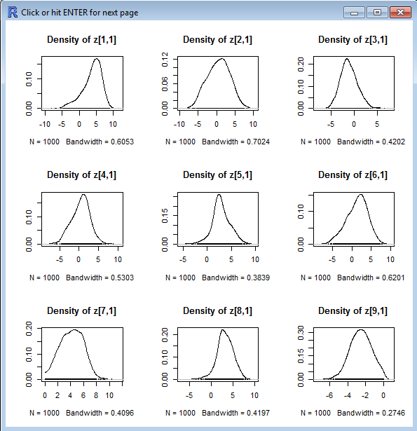
Examine the posterior densities of the paramters, as below:

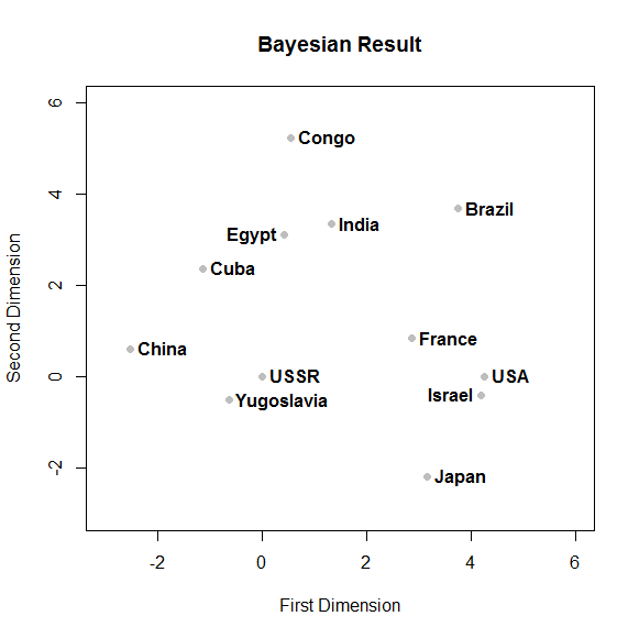
Here is a plot of the Nations from JAGS:

- Run the R program above and
put the Node Statistics Table into WORD NEATLY
FORMATTED! Paste in the Densities for Sigma,
sumllh2, and tau. Show every multi-mode coordinate density and
identify the country.
- Neatly graph the mean coordinates from your
JAGS run and turn in the R code you used to make the plot.
In this Problem we are going to use JAGS to analyze the famous candidate by candidate correlation matrix computed by
Weisberg and Rusk which we used in Weisberg_and_Rusk_Shepard_Plot_2015A.r.
Download the R
program and the text files it uses:
 JAGS_mds_W_and_R.r
-- Program to run the Log-Normal Bayesian Model on the Weisberg and Rusk 1968 Correlation
data.
- Run the R program above and
put the Node Statistics Table into WORD NEATLY
FORMATTED! Paste in the Densities for Sigma,
sumllh2, and tau. Show every multi-mode coordinate density and
identify the candidate.
- Neatly graph the mean coordinates from your
JAGS run and turn in the R code you used to make the plot.
Work Problem (4) on pages 144-145 of Analyzing Spatial Models of Choice and Judgment with R. You will
need the files posted on the Armstrong et al. book chapter 4 website. In particular,
an agreement score matrix and the
JAGS model file.
 JAGS_mds_nations.r
-- Program to run the Log-Normal Bayesian Model on the Nations
data.
 JAGS_mds_model.bug
-- Model used by JAGS
 nations.Rda
-- Nations Data used by JAGS

 JAGS_mds_W_and_R.r
-- Program to run the Log-Normal Bayesian Model on the Weisberg and Rusk 1968 Correlation
data.
 JAGS_mds_W_R_model.bug
-- Model used by JAGS
 nes1968_first_11.dta
-- Stata 11 File for the 1968 National Election Study. Data drawn from Stata file.