---

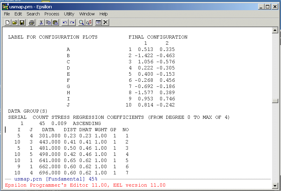
1. In this problem we are going to make a Shepard Diagram (see Borg and Groenen p. 43) for the two dimensional coordinates of the U.S. Map Driving Distance Data. We are going to use the "Printer Output File" for the "REGRESSION=ASCENDING" run you did for 3(b) for homework one. Bring the file up in Epsilon and page down until you are just below the two-dimensional coordinates for the 10 cities. You should see the following:
   
   
   
   The columns we need are below the labels "DATA", "DIST", and "DHAT". We are going to extract these from the file and write them to a text file that we can then read into R. To do this we are going to write a simple Epsilon macro. First, split the screen:
   
   C-X 2 (Split Window Command)
   
   Now use the
   
   C-X C-F (Find File Command)
   
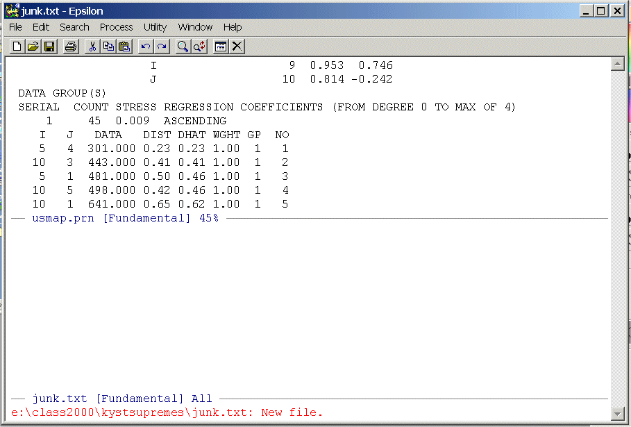
   command to get an empty file -- junk.txt. You should see:
   
   
   
   Highlight the data from the line below the labels on down -- there will be 45 rows -- and put it on the clipboard. Now close the upper window
   
   C-X 0 (Removing/Creating Windows Command)
   
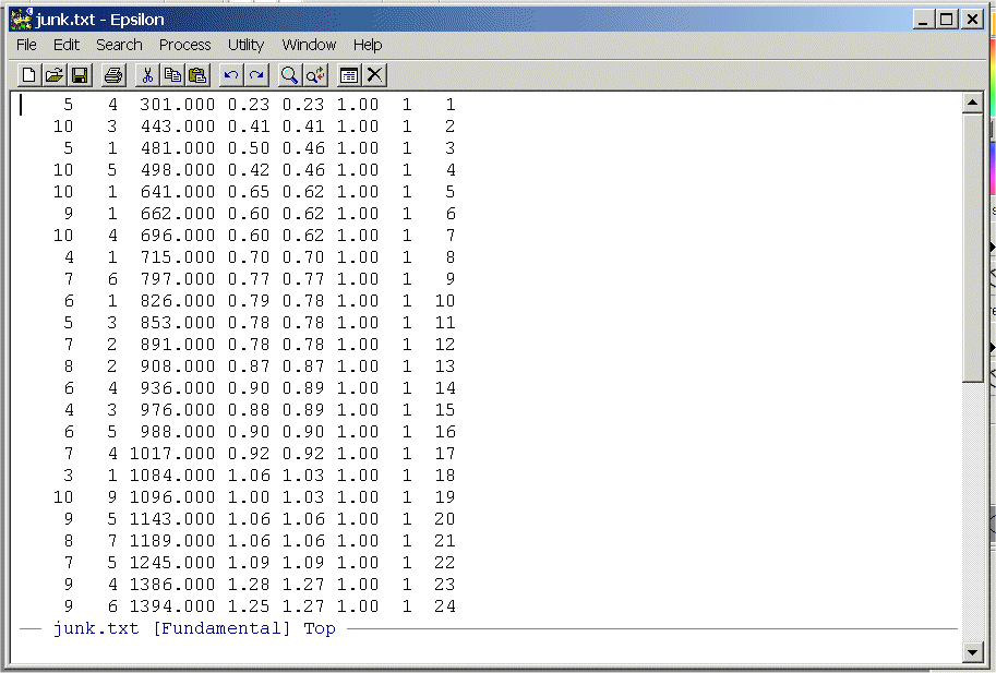
   and paste it into junk.txt, save junk.txt, and position the cursor at the top of the file. You should see:
   
   
   
   
   1. Write a simple Epsilon macro to remove the first two columns and the last three columns. List your commands and turn them in.
      
      
   2. Use the following R program to make the Shepard Plot:
      
      Shepard_Plot_Driving_Distances.r
      
      Here is what the program looks like:

      
      #
      #
      #
      #  Shepard_Plot_Driving_Distances.r -- Does Shepard Plot of Driving Distances
      #                                       for Cities Problem in Homeworks 1 and 2
      #                                       UCSD 2006
      #
      #  
      #  Remove all objects just to be safe
      #
      rm(list=ls(all=TRUE))
      library(MASS)
      #
      T <- matrix(scan("C:/uga_course_homework_2/driving_distances_ordered.txt",0),ncol=3,byrow=TRUE)
      #                          You Created this in Question 1a
      nrow <- length(T[,1])
      ncol <- length(T[1,])
      #                                                      This sets up a plot with the horizontal axis
      plot(T[,1], T[,2],type="n",main="",xlab="",ylab="",     being the observed data (DATA) and vertical axis
               xlim=c(0,3200),ylim=c(0,3),font=2)             being the reproduced distances (DIST)
      points(T[,1], T[,2],pch=16,col="red",cex=1.2)          This Plots the Distances (DIST)
      points(T[,1], T[,3],pch=16,col="blue",cex=1.2)         This Plots the D-HATs (DHAT)
      #
      #  The "S" means "stair-steps"
      #
      lines(T[,1], T[,3],lty=1,lwd=2,type = "S",font=2)  Draws lines between points essentially in
      #                                                    "city block" style
      # Main title
      mtext("Shepard Diagram for Driving Distances",side=3,line=1.00,cex=1.2,font=2)  Side 3 = Top
      # x-axis title
      mtext("Observed Dissimilarities",side=1,line=2.75,font=2,cex=1.2)  Side 1 = bottom
      # y-axis title
      mtext("Estimated Dissimilarities (D-hats)",side=2,line=2.75,font=2,cex=1.2) Side 2 = left side
      #
      

      Note that the stairstep plot is almost perfect. We can see this by computing the Pearson correlation between the driving distances (DATA) and the distances from the spatial map (DIST). This can be done with the simple R Command:
      
      cor(T[,1],T[,2])
      
      Compute this correlation and the one between the driving distances and the DHAT's from the Monotone Regression. Report the correlations and turn in the Plot.
      
      
2. Make Shepard plots of the Morse Code data (both Lower Half and Upper Half) from Question 4) of homework one. Modify the R code above to make the plots. Turn in the plots, the R codes, and the Pearson correlations between DATA and DIST and DATA and DHAT.
   
   
3. R has a MDS program and we will now see if we can duplicate some of our results using it starting with the Cities Problem from Question 3) of homework one. Download
   
   Drive_MDS.r
   
   driver_2_full.txt -- Symmetric Matrix of Driving Distances
   
   Here is what the program looks like:

   
   #
   #
   #
   #  Drive_MDS.r -- Set up to do Simple MDS on Driving Distance Data
   #
   # ATLANTA      0000 2340 1084  715  481  826 1519 2252  662  641
   # BOISE        2340 0000 2797 1789 2018 1661  891  908 2974 2480
   # BOSTON       1084 2797 0000  976  853 1868 2008 3130 1547  443
   # CHICAGO       715 1789  976 0000  301  936 1017 2189 1386  696
   # CINCINNATI    481 2018  853  301 0000  988 1245 2292 1143  498
   # DALLAS        826 1661 1868  936  988 0000  797 1431 1394 1414
   # DENVER       1519  891 2008 1017 1245  797 0000 1189 2126 1707
   # LOS ANGELES  2252  908 3130 2189 2292 1431 1189 0000 2885 2754
   # MIAMI         662 2974 1547 1386 1143 1394 2126 2885 0000 1096
   # WASHINGTON    641 2480  443  696  498 1414 1707 2754 1096 0000
   #  
   #  Remove all objects just to be safe
   #
   rm(list=ls(all=TRUE))
   library(MASS)
   #
   T <- matrix(scan("C:/uga_course_homework_2/driver2_full.txt",0),ncol=10,byrow=TRUE)
   maxT <- max(T)            This finds the maximum entry in the 10 by 10 Matrix T
   T <- T/maxT               This makes the maximum entry in T = 1.0
   #                         This is handy because the R KYST Program does not like large Distances!
   nrow <- length(T[,1])
   ncol <- length(T[1,])
   #
   #
   #  Labels For Cities      This is Just like problem 2) of Homework 1 -- Supreme Court Plot
   #
   junk <- NULL
   junk[1] <- "Atlanta"
   junk[2] <- "Boise"
   junk[3] <- "Boston"
   junk[4] <- "Chicago"
   junk[5] <- "Cincinnati"
   junk[6] <- "Dallas"
   junk[7] <- "Denver"
   junk[8] <- "Los Angeles"
   junk[9] <- "Miami"
   junk[10] <- "Washington"
   #
   namepos <- rep(2,nrow)    This is Just like problem 2) of Homework 1 -- Supreme Court Plot
   #
   namepos[1] <- 2    # Atlanta
   namepos[2] <- 2    # Boise
   namepos[3] <- 2    # Boston
   namepos[4] <- 2    # Chicago
   namepos[5] <- 2    # Cincinnati
   namepos[6] <- 2    # Dallas
   namepos[7] <- 2    # Denver
   namepos[8] <- 2    # Los Angeles
   namepos[9] <- 2    # Miami
   namepos[10] <- 2   # Washington
   #
   #  Call Classical Kruskal-Young-Shepard-Torgerson Non-Metric 
   #           Multidimensional Scaling Program
   #
   # T -- Input
   # dim=2 -- number of dimensions
   # y -- starting configuration (generated internally)
   #
   #  Scale in two dimensions
   #
   kdim <- 2                 Set the Number of Dimensions
   y <- rep(0,kdim*ncol)     The Program wants to see the matrix y so
   dim(y) <- c(ncol,kdim)       we create it here
   #
   #  Call Kruskal NonMetric MDS
   #
   drivenmds <- isoMDS(T,y=cmdscale(T,kdim),kdim, maxit=50)  Here is the call to KYST.  Note that 
   #                                                           we store the output in the data
   #                                                           structure drivenmds:
   #  PLOT FUNCTIONS HERE                                      drivenmds$points[,kdim]
   #                                                           drivenmds$stress -- multiply by 0.01
   #
   # Main title       Your Plot will be like this:
   #                  plot(drivenmds$points[,1],drivenmds$points[,2],type="n",asp=1,etc etc
   #
   mtext("City Map",side=3,line=1.00,cex=1.2,font=2)
   # x-axis title
   mtext("",side=1,line=2.75,font=2,cex=1.2)
   # y-axis title
   mtext("",side=2,line=2.75,font=2,cex=1.2)
   #
   #
   

   Modify this program to make a nice looking plot of the cities. Turn in the plot and the final version of the above R program you develop to do the plot.