and the sample data file
and place them in the same folder on a WINTEL machine.
The sample data file is reproduced below. It contains the lower half of an agreement score matrix computed between the 31 supreme court justices who served on the court from 1945 to 2000.
TORSCA                   Method to get initial starting configuration
PRE-ITERATIONS=3         Number Iterations to Improve starting config.
DIMMAX=2,DIMMIN=1        Maximum & Minimum Number of Dimensions
COORDINATES=ROTATE       Rotate Coordinates so Principal Components lie along axes
ITERATIONS=25            Maximum Number of Iterations
REGRESSION=DESCENDING    Monotone Regression for Similarities -- NONMETRIC MDS
DATA,LOWERHALFMATRIX,DIAGONAL=PRESENT,CUTOFF=.01 Anything below .01 is Missing Data
U. S. SUPREME COURT AGREEMENT SCORES Title
 32  1  1                32 = # of Justices, Always set the next two numbers = 1
(12X,101F3.0)            Format Statement For Dataset
BURGER      100
BLACKMUN     81100
POWELL       86 80100
REHNQUIS     87 72 83100
STEVENS      71 77 74 67100
OCONNOR      88 72 86 87 71100
SCALIA      -99 66 85 89 65 85100
KENNEDY     -99 70-99 88 70 86 87100         -99 is the Missing Data Code
SOUTER      -99 72-99 78 75 81 77 84100
THOMAS      -99 55-99 86 56 81 92 82 72100
GINSBURG    -99 67-99 73 80 75 70 79 87 67100
BREYER      -99-99-99 70 78 77 64 75 84 63 84100
RUTLEDGE    -99-99-99-99-99-99-99-99-99-99-99-99100
MURPHY      -99-99-99-99-99-99-99-99-99-99-99-99 86100
VINSON      -99-99-99-99-99-99-99-99-99-99-99-99 63 64100
HARLAN       81 78-99-99-99-99-99-99-99-99-99-99-99-99-99100
BLACK        67 69-99-99-99-99-99-99-99-99-99-99 85 85 63 58100
DOUGLAS      39 42 42 33-99-99-99-99-99-99-99-99 78 79 59 50 77100
STEWART      77 75 80 74 75-99-99-99-99-99-99-99-99-99-99 78 67 58100
MARSHALL     54 65 57 46 65 51 50 50 53-99-99-99-99-99-99 70 66 70 69100
BRENNAN      53 64 56 46 65 52 51 52100-99-99-99-99-99-99 66 76 76 70 91100
WHITE        80 76 79 77 69 77 79 80 76 74-99-99-99-99-99 74 73 56 76 59 64100
WARREN      -99-99-99-99-99-99-99-99-99-99-99-99-99-99-99 60 81 79 71 90 91 79100
CLARK       -99-99-99-99-99-99-99-99-99-99-99-99-99-99 91 74 67 61 77-99 77 83 77100
FRANKFUR    -99-99-99-99-99-99-99-99-99-99-99-99 58 61 70 86 60 55 79-99 67-99 63 71100
WHITTAKE    -99-99-99-99-99-99-99-99-99-99-99-99-99-99-99 81 57 52 82-99 66-99 62 75 80100
BURTON      -99-99-99-99-99-99-99-99-99-99-99-99 62 58 83 77 60 56-99-99 65-99 66 81 72 80100
REED        -99-99-99-99-99-99-99-99-99-99-99-99 65 62 84 67 60 60-99-99 69-99 71 82 67-99 82100
FORTAS      -99-99-99-99-99-99-99-99-99-99-99-99-99-99-99 63 68 76 72 89 87 75 85 74-99-99-99-99100
GOLDBERG    -99-99-99-99-99-99-99-99-99-99-99-99-99-99-99 59 78 80 77-99 90 78 87 71-99-99-99-99-99100
MINTON      -99-99-99-99-99-99-99-99-99-99-99-99-99-99 87 72 62 57-99-99-99-99 75 84 68-99 82 83-99-99100
JACKSON     -99-99-99-99-99-99-99-99-99-99-99-99 57 57 75-99 57 53-99-99-99-99 75 78 80-99 74 73-99-99 73100
COMPUTE                 These two Lines
STOP                    Must Always be Included
You must run the program from a DOS Window. To run the program type:
KYSTBIG
The program will then prompt you for three file names: the name of the data file (it calls this the "Control Card File"); the name of an output file that you can then print out; and the name of the file for the coordinates.
Control Card File? SUPKYST.DAT
Printer Output File? SUPREME.PRN
Coordinate Output File? SUPS.DAT
The program then runs the analysis and writes the output files to disk.
The first part of this homework problem is to produce a two dimensional graph of the coordinates that are in the SUPS.DAT. To do this The first step is to use Epsilon to insert the names from the SUPKYST.DAT file into SUPS.DAT. Open SUPS.DAT with Epsilon. Type
C-X 2 -- This means "Hold the Control key down and type X and then type 2" (The Split Window Command in Epsilon)
You should see the following:
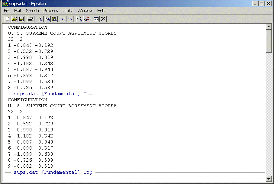
Note that your cursor will be in the bottom screen. Now we want to place SUPKYST.DAT in the bottom screen. To do this, use the command:
C-X C-F -- This means "Hold the Control key down and type X then hold the Control key down and type F"
You will see:
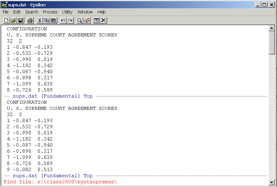
This is the "Find file" command and Epsilon will default to whatever directory that you are currently using. Your cursor will be at the end of path statement -- in my case C:\class2000\kystsupremes\ -- but you can type in any path statement you want. Since this is the directory that contains SUPKYST.DAT, we simply type that at the end of the path statement like this:
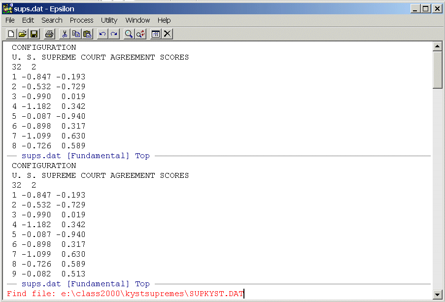
Now, just hit the Enter key and you should see:
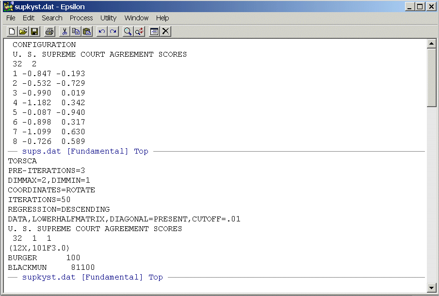
Before continuing with the problem, you will sometimes want to find a file but you have forgotten the name. Suppose, however, you know what directory it is in. In the above, instead of typing SUPKYST.DAT at the end of the path statement, try simply hitting the Enter key. You will see:
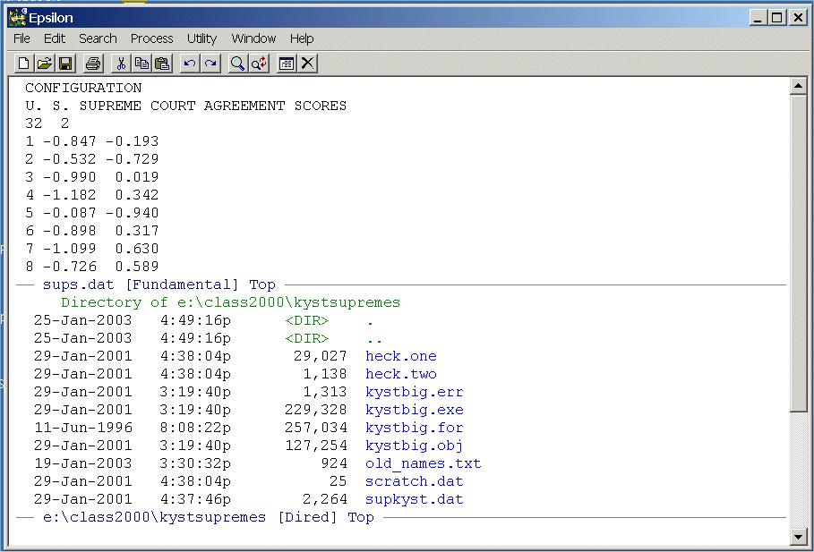
Epsilon lists all the files in the directory and the cursor will be positioned at the top. You can use the down and up arrow keys to move up and down the file list. Position the cursor at the beginning of the file you want and hit the Spacebar. The file will appear in the bottom window just as above. To close the screen your cursor is in you can use the command:
C-X 0 -- This means "Hold the Control key down and type X then type 0 (zero not ohh)"
To close all screens except the one your cursor is in, you can use the command:
C-X 1 -- This means "Hold the Control key down and type X then type 1"
What we are going to do next is write a macro that will take the names of the justices from the SUPKYST.DAT file and insert them into the coordinates embedded in SUPS.DAT. Since this will alter SUPS.DAT, we can use Epsilon to make a copy of the file that we can safely edit. To do this, you need to have the cursor in the upper screen. To toggle back and forth between screens use the command:
C-X o -- This means "Hold the Control key down and type X then type o (this is ohh, not zero!)"
This will move the cursor to the top screen. Now we are going to write a copy of SUPS.DAT to disk and we will call it SUPREME_NAMES.TXT. Type the command:
C-X C-W -- This means "Hold the Control key down and type X then hold the Control key down and type W"
You will see:
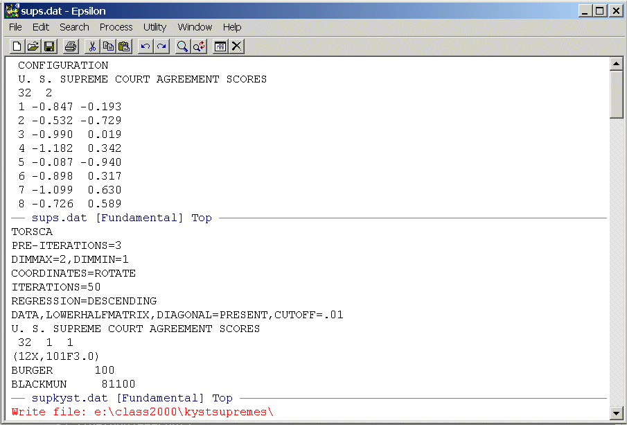
Note the Write File: at the bottom of the screen. This is exactly like the "Find file" command above. Type the name of the file you want to write to at the end of the path statement -- in our case -- SUPREME_NAMES.TXT -- and hit the Enter key. You should see this:
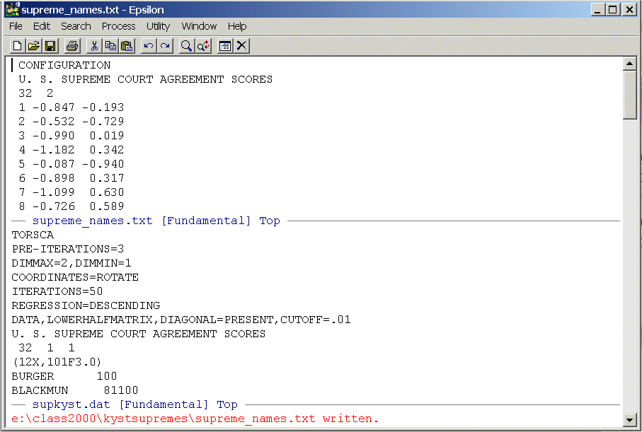
Note that the name of the file in the top screen has changed to supreme_names.txt. Now, delete everything in the file except the two dimensional coordinates. To do this, simply highlight the rows of the file (use the normal WINDOZE key combination of shift-down-arrow or shift-up-arrow) you want to delete and hit the Delete key. Position your cursor at the top of the screen to the far left. We are now going to write an Epsilon macro (to see a helpful example of a macro go through Advanced Multivariate Homework 3 from 2001). Before we begin, use the C-X o command to go down into the lower screen and position the cursor so that it is in front of justice Burger's name (see the Selecting Windows Commands In the Epsilon Manual). Return to the upper screen using the C-X o command. To begin the macro, type:
C-X ( -- This means "Control-X" then "("
You will see:
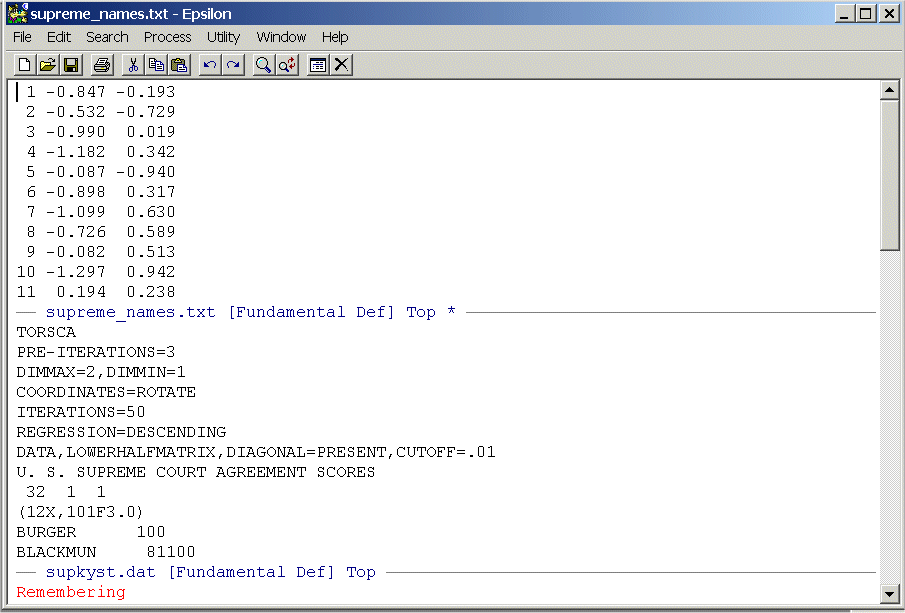
Note the Remembering at the bottom of the screen. Epsilon now records all the key-strokes that you enter until you give the command C-X ). (Also note the asterisk "*" to the far right of the name line at the bottom of the top screen. This is a signal from Epsilon that the file has been altered and not saved. If you clicked on "File Save" that asterisk will not be there.) We will not need the numbers 1 to 32 that are before the two dimensional coordinates. So enter the command:
C-D C-D -- This means "Control-D" twice. Note that this is exactly the same as hitting the Delete key twice.
You should see:
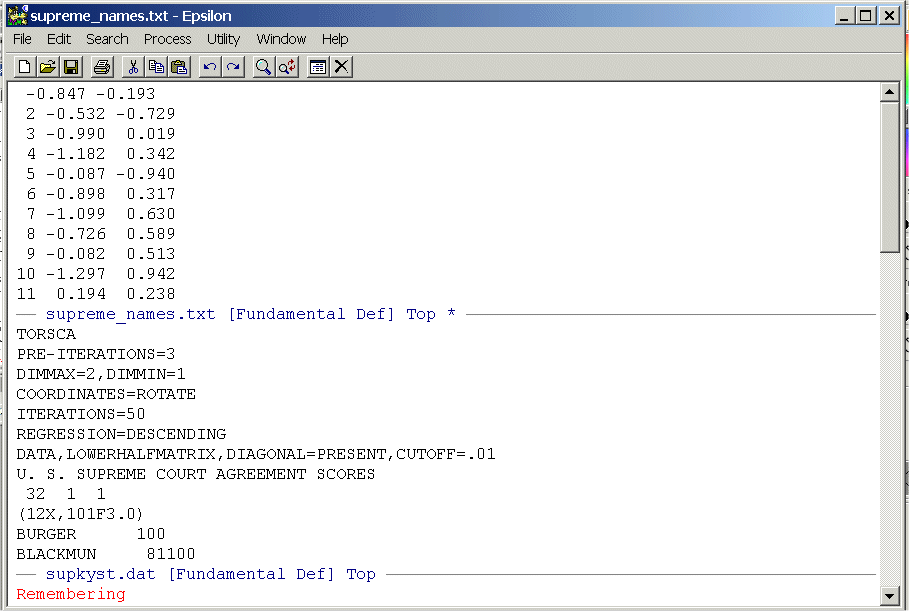
Now we are going down to the lower screen to pick up the names. To do this, first type:
C-X o to go to the lower screen, then type
C-F 12 times.
Your cursor will be right next to the "100" (C-F is the same as Right-Arrow.) Now type:
Enter
And you should see:
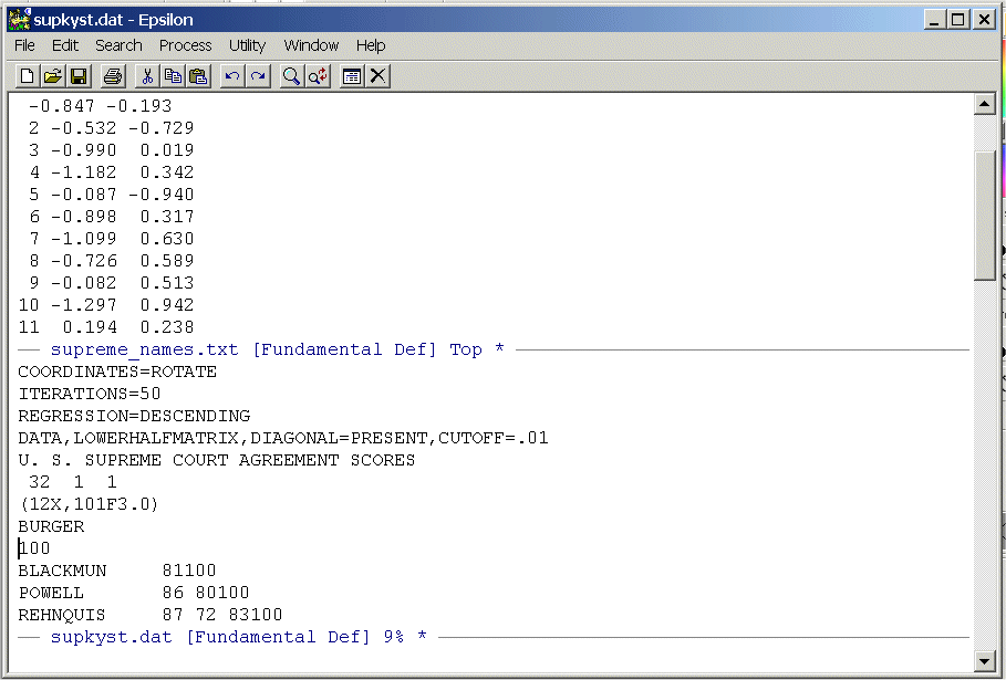
Now, enter the following commands one at a time:
C-P This moves the cursor up one line so it is once again in front of "Burger"
C-K Note that "Burger" disappears -- this places it in the "Kill Buffer"
C-Y Viola, it disgorges it -- this "Yanks" the text from the buffer (the cursor will be at the end)
C-D This re-assembles the original line.
C-A This takes the cursor to the beginning of the line
C-N This positions the cursor at the beginning of the line below. We need to do this so that when the macro runs the first time it gets Blackmun, not Burger!!
C-X o Go back up to the top screen
C-Y Yank Burger from the buffer
C-A Go to the beginning of the line
C-N Position the cursor at the beginning of the line below
C-X ) This ends the remembering and completes the macro.
You should see:
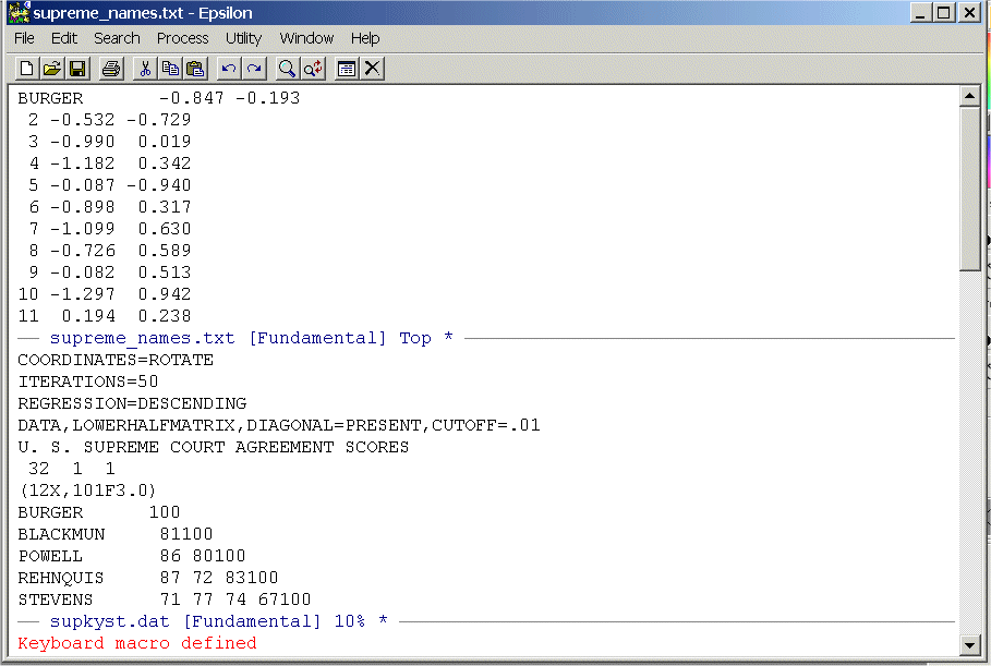
To execute the macro one time type:
C-X E -- This means "hold the Control key down and type X then type E"
You should see:
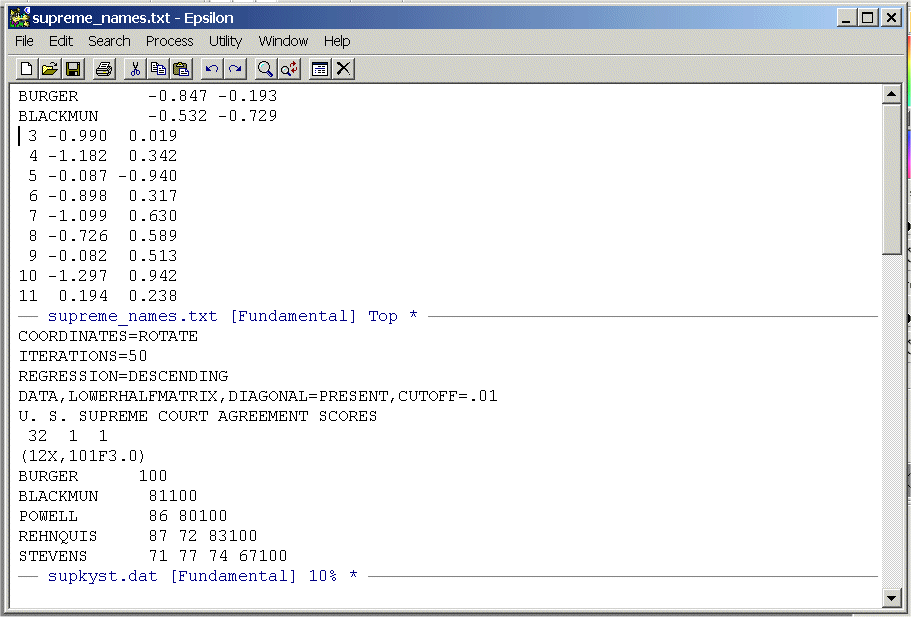
Before executing the macro multiple times it is always good practice to check how many lines there are in the file so that you do not try to go beyond the end of the file (which can have some pretty nasty consequences). To do this type:
C-X L -- This means "hold the Control key down and type X then type L"
You should see:
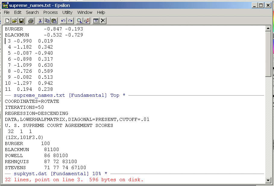
Epsilon tells you that there are 32 lines and the cursor is on line 3. We need to run the macro 30 times but lets execute it only 29 times just to be on the safe side (this is good practice!). To do this type:
C-U -- Control-U. You should see:
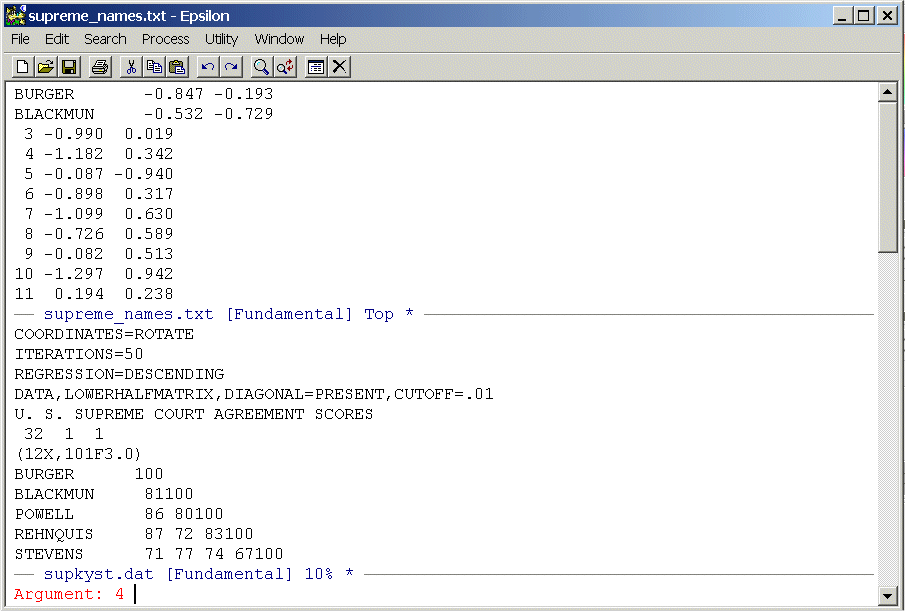
The C-U function will cause whatever command you enter next to be repeated. The "4" is a default. Simply type:
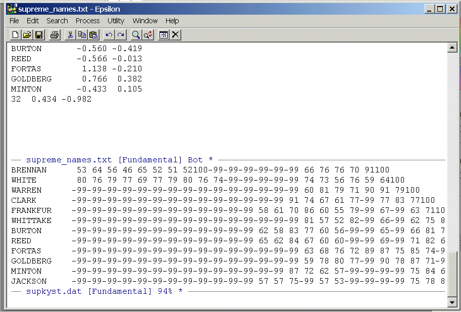
29 C-X E
You should see:
Now, simply execute the macro one more time and you are done:
C-X E
Your cursor should be right below Jackson. We no longer need SUPKYST.DAT so close the lower screen by typing (as described above):
C-X 1
Now save the file in the normal WINDOZE fashion by clicking the floppy token. You can also do this by typing the command:
C-X C-S
Now, place the cursor back at the top of the file. You can do this by simply using the Page-Up but try the command:
ESC < -- This means "hit the Escape key then hit the < (less than) key.
To go to the bottom of the file use the command:
ESC >
(Note that the two commands are the same as:
ALT-< -- Hold down the ALT key and type< (less than).
ALT-> -- Hold down the ALT key and type> (greater than).)
To make our graph in R look good we need to change the names in our file from all caps to just the first letter capitalized. Fortunately, Epsilon has a command:
ALT C -- this means "Hit the "ALT" key then hit "C"
If the cursor is placed right before a word like "BURGER" it will change it to "Burger". You can do this for all 32 justices by writing a simple macro:
C-X (
ALT C
C-A
C-N
C-X )
Execute this for all 32 justices and save the file. You should see:
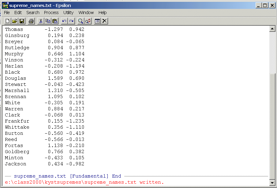
Now exit Epsilon. It will complain because SUPKYST.DAT is still sitting in a buffer and has not been saved. You will see this:
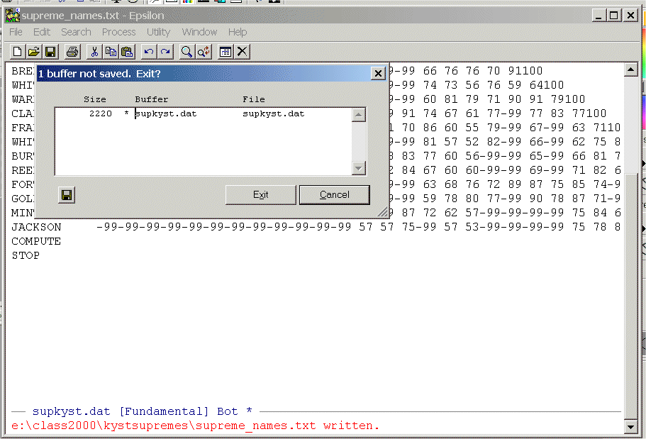
Click on "Exit" and it will flush the altered version of SUPKYST.DAT from its buffer and quit. If you look at SUPKYST.DAT on your disk drive it will be unaltered.
Now, start R
and enter the command:
supremesnames <- read.table("C:/class2000/kystsupremes/supreme_names.txt",header=F,row.names=1)
This tells R to read in the file you just created.
(Be sure to correctly type in the correct path statement!) The "header=F" tells
R that we do not have labels for the
columns and the "row.names=1" tells R that the
first column are row labels. Now type:supremenames
and you should see:
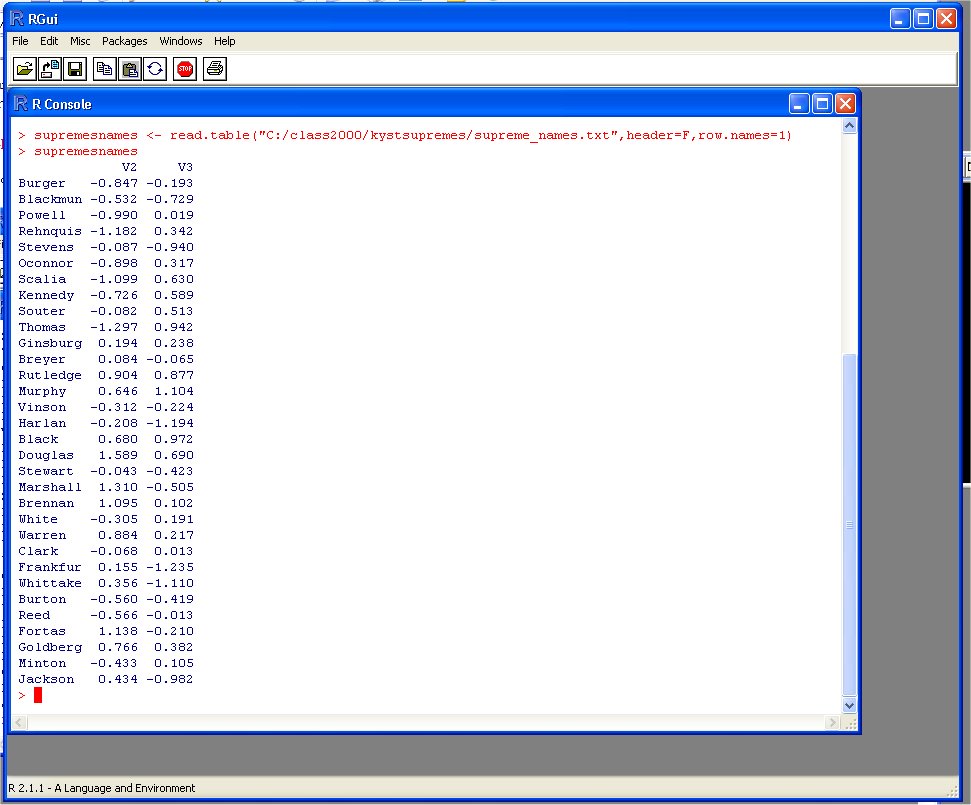
Note that R puts the default headers "V2" and "V3" above the coordinate columns! Now enter the commands:
attach(supremesnames) -- This tells R that you want to work with the columns in "supremesnames"
plot(V2,V3)
text(V2,V3,labels=row.names(supremesnames),adj=0) -- This sticks the names into the plot!
- Turn in the above plot.
- Note that R has chopped off the names
on the right side. We can fix this by telling R
to change the scale of the axes. To do this enter the commands:
plot(V2,V3,xlim=c(-2,2),ylim=c(-2,2))
text(V2,V3,labels=row.names(supremesnames),adj=0)
Turn in the above plot.
- The labels of our axes are lame! Bring up Supreme_names.txt in
Epsilon and insert your own column names. To be
safe, use something short with no spaces so the file looks something like this:
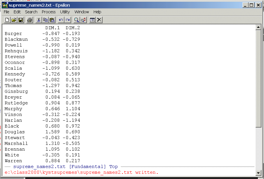
Note that I have saved it as a new file supreme_names2.txt!!
Repeat the steps above only now you need to tell R that you have your own column names. Use the command:
supremesnames2 <- read.table("C:/class2000/kystsupremes/supreme_names2.txt",row.names=1)Replicate (a) and (b) above and turn in the plots.
- In light of what you know about American Politics, do these plots make sense?
#   The cross-hatch is used as a comment marker -- R ignores the line
# plot_supremes.r -- Does a graph of the 32 Supremes using KYST output
#                       file supreme_names.txt    Always put the name of the program at the top
#
# Burger       -0.847 -0.193    This is not necessary but I have no memory
# Blackmun     -0.532 -0.729    so I always put in the file if its small so
# Powell       -0.990  0.019    I do not forget what I am doing!
# Rehnquis     -1.182  0.342
# Stevens      -0.087 -0.940
# Oconnor      -0.898  0.317
# Scalia       -1.099  0.630
# Kennedy      -0.726  0.589
# Souter       -0.082  0.513
# Thomas       -1.297  0.942
# Ginsburg      0.194  0.238
# Breyer        0.084 -0.065
# Rutledge      0.904  0.877
# Murphy        0.646  1.104
# Vinson       -0.312 -0.224
# Harlan       -0.208 -1.194
# Black         0.680  0.972
# Douglas       1.589  0.690
# Stewart      -0.043 -0.423
# Marshall      1.310 -0.505
# Brennan       1.095  0.102
# White        -0.305  0.191
# Warren        0.884  0.217
# Clark        -0.068  0.013
# Frankfur      0.155 -1.235
# Whittake      0.356 -1.110
# Burton       -0.560 -0.419
# Reed         -0.566 -0.013
# Fortas        1.138 -0.210
# Goldberg      0.766  0.382
# Minton       -0.433  0.105
# Jackson       0.434 -0.982
#
#
#  Remove all objects just to be safe
#
rm(list=ls(all=TRUE))  This is not strictly necessary but I do not trust R
#
library(MASS)          This is a standard R library
#
#
#
#  %%%%%%%%%%%%%%%%%%%%%%%%%%%%%%%%%%%%%%%   The next set of commands read the file.
#  Read supreme_names.txt                    This is admitedly clunky way of doing things
#  %%%%%%%%%%%%%%%%%%%%%%%%%%%%%%%%%%%%%%%   but it is bulletproof if you are careful.
#
rcx.file <- "c:/ucsd_homework_1/supreme_names.txt"  Path to the File -- You need the quotes.
#
# Standard fields and their widths -- OC output Legislators
#
rcx.fields <- c("name","dim1","dim2")   You need to name the columns.
rcx.fieldWidths <- c(8,11,7)            You need to give it the exact widths of the columns
#
# Input Legislator Coordinates
#
T <- read.fwf(file=rcx.file,widths=rcx.fieldWidths,as.is=TRUE,col.names=rcx.fields) The Read Statement
dim(T)                   This Turns it into an R dataframe (which looks like a matrix)
#T <- as.matrix(T)       If you do not have any text in the dataset this command
#                        is handy because it makes your input data a true matrix and not a dataframe
names <- T[,1]
dimension1 <- T[,2]      These three commands just make life easier -- they are
dimension2 <- T[,3]      not necessary
#
#
nrow <- length(T[,1])    Here is how you can figure out the number of variables
ncol <- length(T[1,])    and the number of columns
#
#
#  This puts more white space
#    on the Right-Hand-Side Margin
#
par(mar=c(4.1,5.1,4.1,5.1))  This controls the margins on all 4 sides of the plot
#
#
plot(dimension1,dimension2,type="n",asp=1,  The "n" says no visible plot; asp=1 means
       main="",                             maintain the aspect ratio
       xlab="",
       ylab="",
       xlim=c(-2.0,2.0),ylim=c(-2.0,2.0))   These have to be the same for asp=1 to work
points(dimension1,dimension2,pch=16,col="red") Plot the Points
axis(1,font=2)                                 Horizontal axis in bold font
axis(2,font=2,cex=1.2)                         Vertical axis in bold font
# Main title
mtext("U.S. Supreme Court 1945-2000",side=3,line=1.00,cex=1.2,font=2)  Side 3 is the top
# x-axis title                                                         line= controls position
mtext("Liberal-Conservative",side=1,line=2.75,cex=1.2)
# y-axis title
mtext("Who the Heck Knows",side=2,line=2.5,cex=1.2)
#
# pos -- a position specifier for the text. Values of 1, 2, 3 and 4,
# respectively indicate positions below, to the left of, above and
# to the right of the specified coordinates
#
namepos <- rep(2,nrow)     This generates a nrow-length vector of 2's
#
#namepos[1] <- 2    # Burger
#namepos[2] <- 2    # Blackmun   I stuck in the Supremes' Names so
#namepos[3] <- 2    # Powell     You can control their positions
#namepos[4] <- 2    # Rehnquis
#namepos[5] <- 2    # Stevens
#namepos[6] <- 2    # Oconnor
#namepos[7] <- 2    # Scalia
#namepos[8] <- 2    # Kennedy
#namepos[9] <- 2    # Souter
#namepos[10] <- 2   # Thomas
#namepos[11] <- 2   # Ginsburg
#namepos[12] <- 2   # Breyer
#namepos[13] <- 2   # Rutledge
#namepos[14] <- 2   # Murphy
#namepos[15] <- 2   # Vinson
#namepos[16] <- 2   # Harlan
#namepos[17] <- 2   # Black
#namepos[18] <- 2   # Douglas
#namepos[19] <- 2   # Stewart
#namepos[20] <- 2   # Marshall
#namepos[21] <- 2   # Brennan
#namepos[22] <- 2   # White
#namepos[23] <- 2   # Warren
#namepos[24] <- 2   # Clark
#namepos[25] <- 2   # Frankfur
#namepos[26] <- 2   # Whittake
#namepos[27] <- 2   # Burton
#namepos[28] <- 2   # Reed
#namepos[29] <- 2   # Fortas
#namepos[30] <- 2   # Goldberg
#namepos[31] <- 2   # Minton
#namepos[32] <- 2   # Jackson
#
text(dimension1,dimension2,names,pos=namepos,offset=00.00,col="blue") This Plots the Names.
#                                       The offset= adjusts how far the name is from the point.
Run the program in R and you should get this: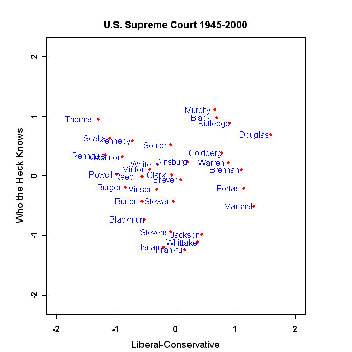
- Produce a nice plot of the Supremes by adjusting the positions of the names
in the namepos[] vector (just delete the "#" at the beginning of the line) and the
offset control. Turn in this plot.
and place it in the same folder with KYST.
The data file is reproduced below. It contains the lower half of a driving distance matrix computed between 10 U.S. cities -- Atlanta, Boise, Boston, Chicago, Cincinnati, Dallas, Denver, Los Angeles, Miami, and Washington, D.C..
PRINT HISTORY, PRINT DISTANCES         This Option Prints out Some Useful Intermediate Output
DIMMAX=3, DIMMIN=1
TORSCA
REGRESSION=POLYNOMIAL=1                METRIC MDS
DATA,LOWERHALFMATRIX,DIAGONAL=PRESENT,CUTOFF=0.0
U.S. MAP EXAMPLE
 10  1  1
(10f5.0)
 0000
 2340 0000
 1084 2797 0000
  715 1789  976 0000
  481 2018  853  301 0000
  826 1661 1868  936  988 0000
 1519  891 2008 1017 1245  797 0000
 2252  908 3130 2189 2292 1431 1189 0000
  662 2974 1547 1386 1143 1394 2126 2885 0000
  641 2480  443  696  498 1414 1707 2754 1096 0000
COMPUTE
STOP
Run this data set through KYST and get the coordinates.
- Modify the Plot_Supremes.r program to make a plot of the 10 U.S. Cities. Turn in a
listing of the program and the two dimensional plot.
- Change REGRESSION=POLYNOMIAL=1 to
REGRESSION=ASCENDING and run it through KYST
(the "ascending"
tells KYST to do a Nonmetric MDS on
dissimilarity data). Compare the
Stress values for 1 to 3 dimensions with those obtained
above and compare the two dimensional plot obtained with this option to that in part (a).
and place it in the same folder with KYST. Here is what MORSEKYSTSL.DAT looks like:
TORSCA
PRE-ITERATIONS=3
DIMMAX=2,DIMMIN=2
PRINT HISTORY,PRINT DISTANCES
COORDINATES=ROTATE
ITERATIONS=50
REGRESSION=DESCENDING
DATA,LOWERHALFMATRIX,DIAGONAL=PRESENT
MORSE CODE DATA -- SIMILARITIES EXAMPLE
 36  1  1
(1X,36F3.0)
A 92  4  6 13  3 14 10 13 46  5 22  3 25 34  6  6  9 35 23  6 37 13 17 12  7  3  2  7  5  5  8  6  5  6  2  3 A
B  5 84 37 31  5 28 17 21  5 19 34 40  6 10 12 22 25 16 18  2 18 34  8 84 30 42 12 17 14 40 32 74 43 17  4  4 B
C  4 38 87 17  4 29 13  7 11 19 24 35 14  3  9 51 34 24 14  6  6 11 14 32 82 38 13 15 31 14 10 30 28 24 18 12 C
D  8 62 17 88  7 23 40 36  9 13 81 56  8  7  9 27  9 45 29  6 17 20 27 40 15 33  3  9  6 11  9 19  8 10  5  6 D
E  6 13 14  6 97  2  4  4 17  1  5  6  4  4  5  1  5 10  7 67  3  3  2  5  6  5  4  3  5  3  5  2  4  2  3  3 E
F  4 51 33 19  2 90 10 29  5 33 16 50  7  6 10 42 12 35 14  2 21 27 25 19 27 13  8 16 47 25 26 24 21  5  5  5 F
G  9 18 27 38  1 14 90  6  5 22 33 16 14 13 62 52 23 21  5  3 15 14 32 21 23 39 15 14  5 10  4 10 17 23 20 11 G
H  3 45 23 25  9 32  8 87 10 10  9 29  5  8  8 14  8 17 37  4 36 59  9 33 14 11  3  9 15 43 70 35 17  4  3  3 H
I 64  7  7 13 10  8  6 12 93  3  5 16 13 30  7  3  5 19 35 16 10  5  8  2  5  7  2  5  8  9  6  8  5  2  4  5 I
J  7  9 38  9  2 24 18  5  4 85 22 31  8  3 21 63 47 11  2  7  9  9  9 22 32 28 67 66 33 15  7 11 28 29 26 23 J
K  5 24 38 73  1 17 25 11  5 27 91 33 10 12 31 14 31 22  2  2 23 17 33 63 16 18  5  9 17  8  8 18 14 13  5  6 K
L  2 69 43 45 10 24 12 26  9 30 27 86  6  2  9 37 36 28 12  5 16 19 20 31 25 59 12 13 17 15 26 29 36 16  7  3 L
M 24 12  5 14  7 17 29  8  8 11 23  8 96 62 11 10 15 20  7  9 13  4 21  9 18  8  5  7  6  6  5  7 11  7 10  4 M
N 31  4 13 30  8 12 10 16 13  3 16  8 59 93  5  9  5 28 12 10 16  4 12  4 16 11  5  2  3  4  4  6  2  2 10  2 N
O  7  7 20  6  5  9 76  7  2 39 26 10  4  8 86 37 35 10  3  4 11 14 25 35 27 27 19 17  7  7  6 18 14 11 20 12 O
P  5 22 33 12  5 36 22 12  3 78 14 46  5  6 21 83 43 23  9  4 12 19 19 19 41 30 34 44 24 11 15 17 24 23 25 13 P
Q  8 20 38 11  4 15 10  5  2 27 23 26  7  6 22 51 91 11  2  3  6 14 12 37 50 63 34 32 17 12  9 27 40 58 37 24 Q
R 13 14 16 23  5 34 26 15  7 12 21 33 14 12 12 29  8 87 16  2 23 23 62 14 12 13  7 10 13  4  7 12  7  9  1  2 R
S 17 24  5 30 11 26  5 59 16  3 13 10  5 17  6  6  3 18 96  9 56 24 12 10  6  7  8  2  2 15 28  9  5  5  5  2 S
T 13 10  1  5 46  3  6  6 14  6 14  7  6  5  6 11  4  4  7 96  8  5  4  2  2  6  5  5  3  3  3  8  7  6 14  6 T
U 14 29 12 32  4 32 11 34 21  7 44 32 11 13  6 20 12 40 51  6 93 57 34 17  9 11  6  6 16 34 10  9  9  7  4  3 U
V  5 17 24 16  9 29  6 39  5 11 26 43  4  1  9 17 10 17 11  6 32 92 17 57 35 10 10 14 28 79 44 36 25 10  1  5 V
W  9 21 30 22  9 36 25 15  4 25 29 18 15  6 26 20 25 61 12  4 19 20 86 22 25 22 10 22 19 16  5  9 11  6  3  7 W
X  7 64 45 19  3 28 11  6  1 35 50 42 10  8 24 32 61 10 12  3 12 17 21 91 48 26 12 20 24 27 16 57 29 16 17  6 X
Y  9 23 62 15  4 26 22  9  1 30 12 14  5  6 14 30 52  5  7  4  6 13 21 44 86 23 26 44 40 15 11 26 22 33 23 16 Y
Z  3 46 45 18  2 22 17 10  7 23 21 51 11  2 15 59 72 14  4  3  9 11 12 36 42 87 16 21 27  9 10 25 66 47 15 15 Z
1  2  5 10  3  3  5 13  4  2 29  5 14  9  7 14 30 28  9  4  2  3 12 14 17 19 22 84 63 13  8 10  8 19 32 57 55 1
2  7 14 22  5  4 20 13  3 25 26  9 14  2  3 17 37 28  6  5  3  6 10 11 17 30 13 62 89 54 20  5 14 20 21 16 11 2
3  3  8 21  5  4 32  6 12  2 23  6 13  5  2  5 37 19  9  7  6  4 16  6 22 25 12 18 64 86 31 23 41 16 17  8 10 3
4  6 19 19 12  8 25 14 16  7 21 13 19  3  3  2 17 29 11  9  3 17 55  8 37 24  3  5 26 44 89 42 44 32 10  3  3 4
5  8 45 15 14  2 45  4 67  7 14  4 41  2  0  4 13  7  9 27  2 14 45  7 45 10 10 14 10 30 69 90 42 24 10  6  5 5
6  7 80 30 17  4 23  4 14  2 11 11 27  6  2  7 16 30 11 14  3 12 30  9 58 38 39 15 14 26 24 17 88 69 14  5 14 6
7  6 33 22 14  5 25  6  4  6 24 13 32  7  6  7 36 39 12  6  2  3 13  9 30 30 50 22 29 18 15 12 61 85 70 20 13 7
8  3 23 40  6  3 15 15  6  2 33 10 14  3  6 14 12 45  2  6  4  6  7  5 24 35 50 42 29 16 16  9 30 60 89 61 26 8
9  3 14 23  3  1  6 14  5  2 30  6  7 16 11 10 31 32  5  6  7  6  3  8 11 21 24 57 39  9 12  4 11 42 56 91 78 9
0  9  3 11  2  5  7 14  4  5 30  8  3  2  3 25 21 29  2  3  4  5  3  2 12 15 20 50 26  9 11  5 22 17 52 81 94 0
COMPUTE
STOP
This is the famous morse code data. If you compare this file to MORSEKYSTSU.DAT they are exactly the same except the matrix is transposed.
- Run MORSEKYSTSL.DAT and MORSEKYSTSU.DAT through KYST (be sure to use
unique output file names) in 1 to 3 dimensions. To do this change:
DIMMAX=2,DIMMIN=2 to
DIMMAX=3,DIMMIN=1
using Epsilon. Report the Stress values for 1 to 3 dimensions for the two halves of the data.
- Make two-dimensional Plots for the two halves of the data (use Epsilon
to put the 26 letters and 10 integers before the corresponding coordinates). (You can modify the
Plot_Supremes.r program to do this.) Turn in the plots and the
R code. Do the plots look the same?