 434_INDIGO        100  86  42  42  18   6   7   4   2   7   9  12  13  16
 445_BLUE           86 100  50  44  22   9   7   7   2   4   7  11  13  14
 465                42  50 100  81  47  17  10   8   2   1   2   1   5   3
 472_BLUE-GREEN     42  44  81 100  54  25  10   9   2   1   0   1   2   4
 490                18  22  47  54 100  61  31  26   7   2   2   1   2   0
 504_GREEN           6   9  17  25  61 100  62  45  14   8   2   2   2   1
 537                 7   7  10  10  31  62 100  73  22  14   5   2   2   0
 555_YELLOW-GREEN    4   7   8   9  26  45  73 100  33  19   4   3   2   2
 584                 2   2   2   2   7  14  22  33 100  58  37  27  20  23
 600_YELLOW          7   4   1   1   2   8  14  19  58 100  74  50  41  28
 610                 9   7   2   0   2   2   5   4  37  74 100  76  62  55
 628_ORANGE-YELLOW  12  11   1   1   1   2   2   3  27  50  76 100  85  68
 651_ORANGE         13  13   5   2   2   2   2   2  20  41  62  85 100  76
 674_RED            16  14   3   4   0   1   0   2  23  28  55  68  76 100
then change the format statement to:
(18X,101F4.0)
Be sure to change the missing values parameter to a negative number because there are some zeroes in the matrix. Your KYST file should look like the following:
TORSCA
PRE-ITERATIONS=3
DIMMAX=3,DIMMIN=1
PRINT HISTORY,PRINT DISTANCES
COORDINATES=ROTATE
ITERATIONS=50
REGRESSION=DESCENDING
DATA,LOWERHALFMATRIX,DIAGONAL=PRESENT,CUTOFF=-.01
EKMAN'S COLOR DATA EXAMPLE
 14  1  1
(18X,101F4.0)
****the color data****
COMPUTE
STOP
-
Run all tables from 3 to 1 dimensions, report the Stress values, and
use R to graph the results for each table in two
dimensions.
Produce Shepard Diagrams for each two dimensional solution (the horizontal axis is the actual similarities data -- the "DATA" column in the KYST output file -- and the vertical axis is the estimated distances -- the "DIST" column in the KYST output file).
(define-macro "hw4" "C-U41C-FC-KC-YC-AC-NC-XoC-XoC-YC-AC-XpC-U19C-FC-MC-PC-KC-YC-DC-AC-NC-XoC-YC-AC-EC-MC-XpC-Xp")
-
Simply highlight the above, put it on the clipboard, and paste it into
Epsilon and save it in the same directory that
you have the output files for the color example.
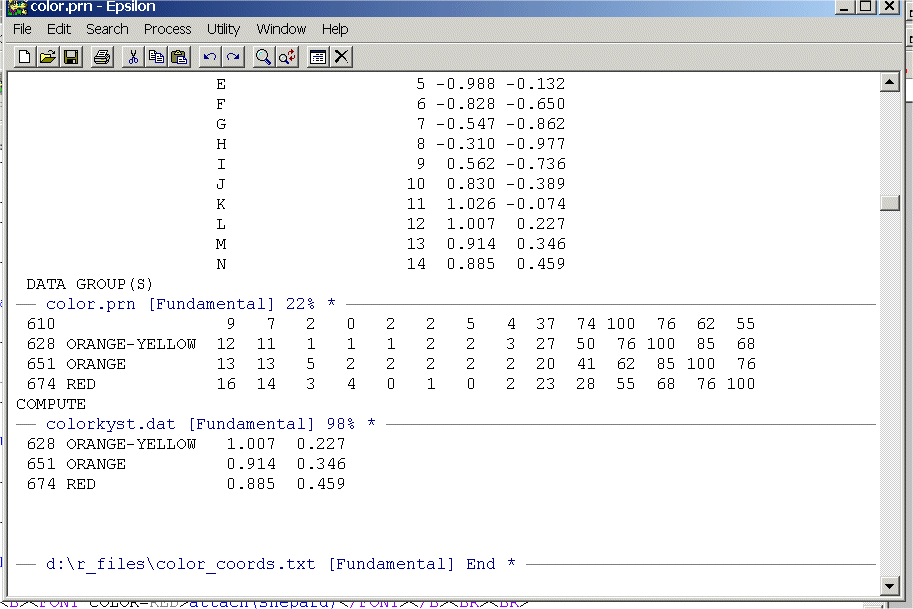
Now, bring up the KYST coordinates in the top window, the color matrix in a center window, and an empty window at the bottom. It should look like this:
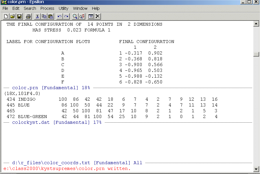
Make sure that you have positioned the cursor in the top window at the beginning of the line for the first set of coordinates and positioned the cursor in the middle window at the beginning of the line "434 INDIGO...".
Now, to load the macro into Epsilon, type:
Alt-X
and you will see Command: appear at the bottom of the screen. Now type:
load-buffer
and you should see:
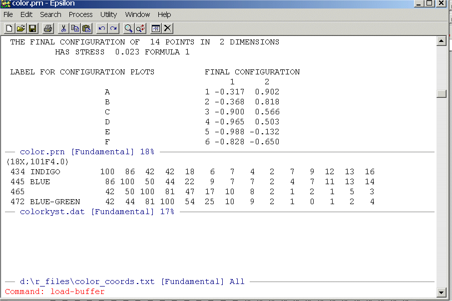
Now hit Enter and type:
macro_hw4.txt
You should see:
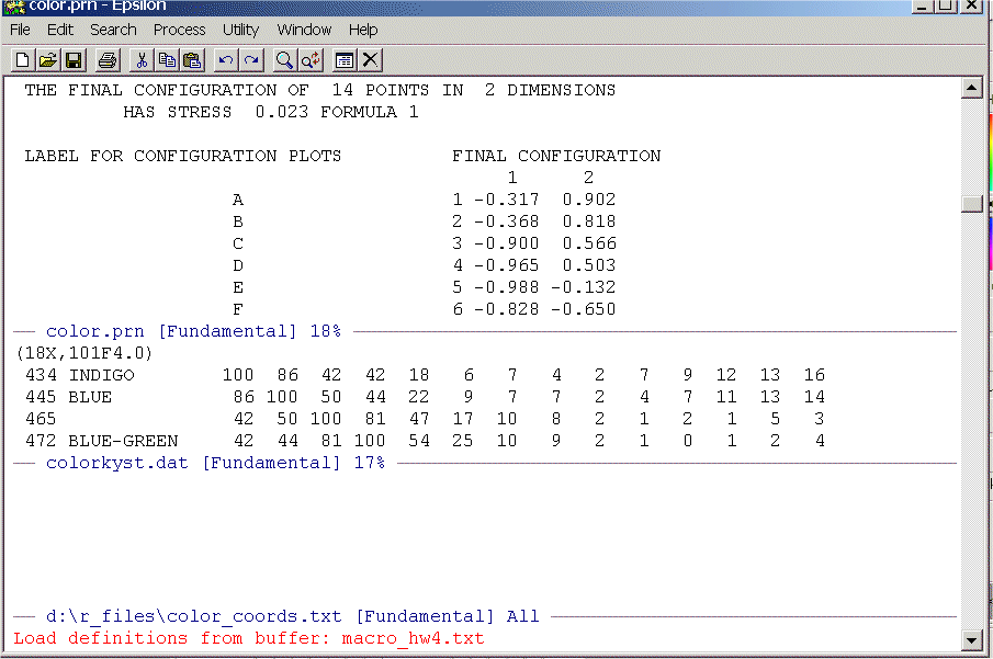
Now hit Enter and you should see the following:
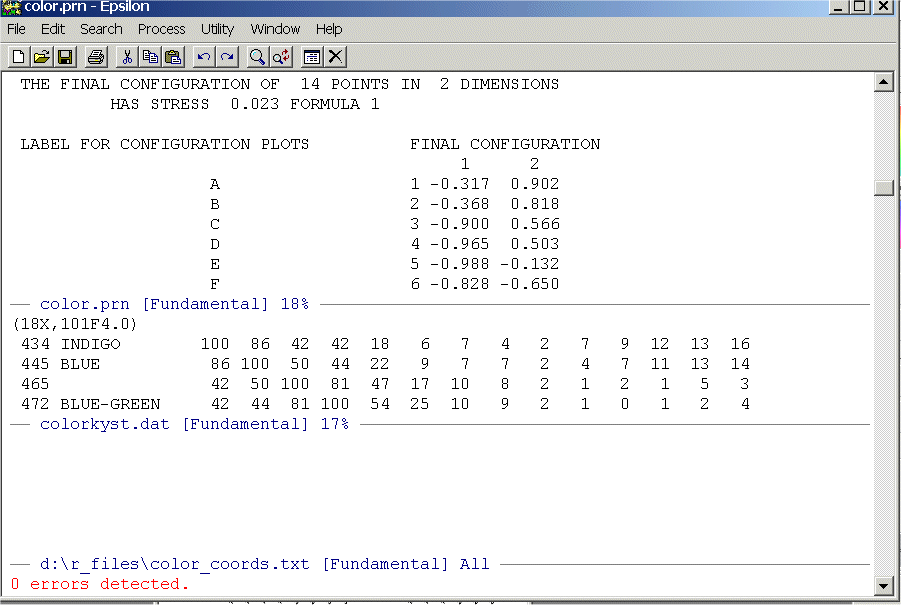
If you see 0 errors detected. then Epsilon is satisifed that the macro is a legal series of commands.
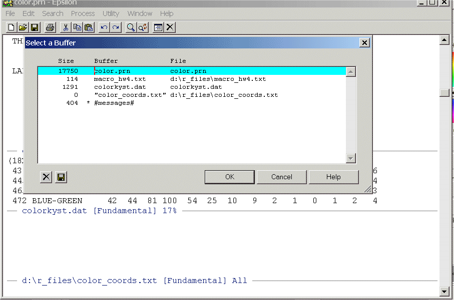
Before continuing with executing the macro, note that above what Epsilon wanted was the name of a buffer -- that is, a file that it has in its buffer list -- this is why you pulled macro_hw4.txt into Epsilon earlier. If you forget the names of files that you have been working with you can always see the list of Epsilon buffers by typing the command at any time:
C-XC-B
And you will see:
To execute the macro one time type:
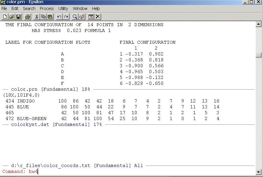
Alt-X then
hw4
You should see:
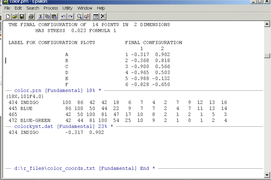
Now hit Enter and the macro executes one time and your screen should show this:
To execute the macro multiple times use the C-U command; namely, do the keystrokes:
C-U13Alt-Xhw4
and you will see:
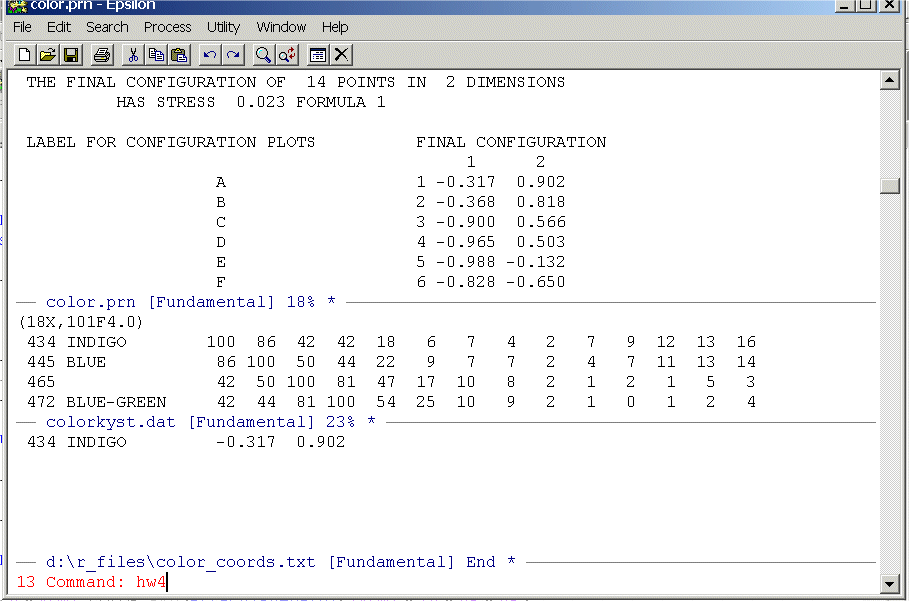
Now hit Enter and you will see:
Save color_coords.txt and close the other two windows. Use Epsilon to type variable labels into your file and also place commas between the variables (we are going to do a new type of read-table in R). Also make sure that everything is in lower-case -- you can use the Alt-L command in Epsilon to do this. Your file should look something like this:
                      DIM.1,  DIM.2
 434_indigo        , -0.317,  0.902
 445_blue          , -0.368,  0.818
 465               , -0.900,  0.566
 472_blue-green    , -0.965,  0.503
 490               , -0.988, -0.132
 504_green         , -0.828, -0.650
 537               , -0.547, -0.862
 555_yellow-green  , -0.310, -0.977
 584               ,  0.562, -0.736
 600_yellow        ,  0.830, -0.389
 610               ,  1.026, -0.074
 628_orange-yellow ,  1.007,  0.227
 651_orange        ,  0.914,  0.346
 674_red           ,  0.885,  0.459
-
Read your coordinate file into R with the
command:
colornames <- read.csv("D:/r_files/color_coords.txt",header=T,row.names=1)
then be sure to attach the file so you can work with the variables:
attach(colornames)
The ".csv" tells R that color_coords.txt is comma delimited! When you set up your coordinate files this way you do not need to use "_" in the labels. But be sure that in the column label line that you have commas separating the labels.
Make a plot of the color coordinates. Set the axes so that you can see the labels and the plot looks nice (the "xlim" and "ylim" commands). You can suppress the "o"'s before the names by using the commands:
plot(DIM.1,DIM.2,type="n",main="The Color Circle",xlim=c(-2,2),ylim=c(-2,2))
text(DIM.1,DIM.2,labels=row.names(colornames),adj=0)
The 'type="n"' suppresses the display of the "o"'s.
Edit macro_hw4.txt so that you can use it to create the coordinate file for Table 1.3 -- the similarities for nations. Call the macro macro_hw4_2b.txt. Turn in this macro and the file that it creates.
                           1   2   3   4   5   6   7
                         ---------------------------
                       1 | 0   2   1   2   2   1   2
                         |
                       2 | 2   0   1   4   8   5   4
                         |
                       3 | 1   1   0   1   5   4   5
                         |
                       4 | 2   4   1   0   4   5   8
                         |
                       5 | 2   8   5   4   0   1   4
                         |
                       6 | 1   5   4   5   1   0   1
                         |
                       7 | 2   4   5   8   4   1   0
                         ---------------------------