LEGACY CONTENT.
If you are looking for Voteview.com, PLEASE CLICK HEREThis site is an archived version of Voteview.com archived from University of Georgia on
May 23, 2017. This point-in-time capture includes all files publicly linked on Voteview.com at that time. We provide access to this content as a service to ensure that past users of Voteview.com have access to historical files. This content will remain online until at least
January 1st, 2018. UCLA provides no warranty or guarantee of access to these files.
45-733 PROBABILITY AND STATISTICS I
The Poisson Distribution
æ [(lx)e-l]/x!
ç
f(x) = ç x=0,1,2,3,4,...
ç
è 0 otherwise
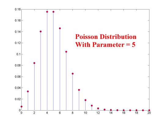
Mean = E(X) = l; and
Variance = VAR(X) = l
where Lambda,
l, is the
average number of occurrences of the
phenomenon in 1 unit of time, space, or volume.
The classic example of the Poisson distribution is the distribution of deaths
in the Prussian Calvary due to horse-kicks to the head. The table below
shows deaths from horse-kicks 10 Army Corps over a 20 year period for a
total of 200 "Corps-Years".
Number Reports
With This
Deaths Many Deaths Proportion
---------------------------------
0 109 .545
1 65 .325
2 22 .110
3 3 .015
4 1 .005
---------------------------------
200 1.000
It is reasonable to assume that deaths from horse-kicks should occur
randomly over time. Consequently, the number per Corps-Year should
have a Poisson distribution. To test this, we can treat the above
data as a random sample and compute the sample mean. Using the sample
mean to estimate l, we can
compute the Poisson probabilities from this l
and compare them to the actual
frequencies in the above table and see how closely they match.
_
Xn = [åi=1,n Xi]/n =
(total deaths)/(200 Corps-Years) =
(0*109 + 1*65 + 2*22 + 3*3 + 4*1)/200 = 122/200 = .61
Using l = .61 produces the following
probabilities:
Number Reports
With This
Deaths Many Deaths Proportion l=.61
----------------------------------------
0 109 .545 .543
1 65 .325 .331
2 22 .110 .101
3 3 .015 .021
4 1 .005 .003
----------------------------------------
200 1.000 .999
Note that only .001 of the Poisson probability is above X=4.
The Poisson Distribution and its
Relationship to the Exponential Distribution
The Poisson Distribution can also be interpreted in the following form:
æ [(lt)xe-lt]/x!
ç
f(x) = ç x=0,1,2,3,4,...
ç
è 0 otherwise
Mean = E(X) = lt; and
Variance = VAR(X) = lt2
where l is, as above, the average
number of occurrences in one unit of time, and t is the length of
the time period.
Let T denote the amount of time until the first occurrence. If
T > t then there must have been no occurrences in the first t units
of time. The probability of this event is:
P(T > t) = P(X = 0)= e-lt
and by the rule of the complement:
P(T £ t) =
1 - e-lt
The distribution function for T is therefore:
æ 0 t < 0
F(t) = ç
è 1 - e-lt t ³ 0
Since this is a continuous function, we can take the derivative and obtain
the distribution:
æ le-lt t ³ 0
f(t) = ç
è 0 otherwise
Where
Mean = E(T) = 1/l; and
Variance = VAR(T) = 1/l2
This is the Exponential Distribution. It is the
distribution of the time until the first occurrence of an event or the
distribution of the amount of time between events where the
occurrences of the phenomenon are governed by a Poisson process.
For example, suppose the arrival of cars at a Turnpike entrance is
governed as a Poisson process with a mean of 3 per minute. Suppose the
ticket taker has to leave the booth for 1 minute. What is the probability
that no cars arrive during the ticket taker's absence?
P(T > 1) = 1 - F(1) = e-3*1 = .04979
As shown by this simple example the Exponential and Poisson distributions
have many useful applications to what are known as
Waiting Time Problems. For example, the arrival of ships
at a port (both number and the time in between the arrivals); the arrival
of freight trains at a classification yard; etc. The examples are legion.