A variable the value of which is a number determined by the outcome of an experiment. Example: We flip a coin. Let X = 1 if Heads, and let X = 0 if Tails. Example: We roll a die. Let X = "number of dots". Definition: Probability Distribution: A function that assigns probabilities to the values of a random variable. Example: We flip a coin. Given the definition of a random variable in (2), let the probability distribution be:
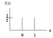
                              æ1/2 x = 0
                              ç
                       f(x) = ç1/2 x = 1
                              ç
                              è 0 otherwise
A plot of this function looks like this:
                              æ1/36  x = 2 or x = 12
                              ç
                              ç2/36  x = 3 or x = 11
                              ç
                              ç3/36  x = 4 or x = 10
                              ç
                       f(x) = ç4/36  x = 5 or x = 9
                              ç
                              ç5/36  x = 6 or x = 8
                              ç
                              ç6/36  x = 7
                              ç
                              è 0 otherwise
Properties of Discrete Probability Distributionsa) f(xi) ³ 0 for all i
b) åi=1,n f(xi) = 1
c) P[a £ X £ b] = å f(xi) Example: With respect to (8):
P[6 £ X £ 9] = P[X = 6] + P[X = 7] + P[X = 8] + P[X = 9] =
1/36(5 + 6 + 5 + 4) = 20/36 = 5/9
Note that: P[6 < X £ 9] = P[7 £ X £ 9]
Definition: Distribution Function
F(x) = P(X £ x) Example: With respect to (8):
F(5) = P[X = 1] + P[X = 2] + P[X = 3] + P[X = 4] + P[X = 5] =
1/36(1 + 2 + 3 + 4) = 10/36 = 5/18 Note that, when working with discrete distributions that:
P[X < 5] = F(4)
P[5 £ X £ 8] = F(8) - F(4)
P[5 £ X < 8] = F(7) - F(4)
P[5 < X < 8] = F(7) - F(5) Discrete Uniform Distribution
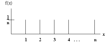
                         æ1/n x = 1,2,3,4,5,...,n
                  f(x) = ç
                         è 0 otherwise
A graph of the function looks like this:
P[X £ 3] = 3/n
P[4 £ X £ n] = 1 - P[X < 4] = 1 - F(3) = (n-3)/n
F(5) = 5/n Bernoulli Distribution
A Bernoulli experiment or trial is an experiment with only two possible outcomes. Traditionally these are known as a success and a failure. Let X = 1 be a success, and X = 0 be a failure, and let p be the probability: P(X = 1). Hence:
                         æ p  x = 1
                         ç
                  f(x) = ç1-p x = 0
                         ç
                         è 0 otherwise
Binomial DistributionLet X1, X2, X3, ..., Xn be random variables corresponding to n Bernoulli trials (experiments), and let Z be the random variable:
Z = åi=1,n Xi
The distribution of Z is the binomial
                         æ ænö
                         ç ç ÷ pz(1-p)(n-z)
                  f(z) = ç èzø          z=0,1,2,3,...,n
                         ç
                         è 0 otherwise
Example: Let n = 4 and p = 1/2, thenP[Z = 2] = (4 choose 2)(1/2)2(1/2)2 = 6/16 = 3/8 Problem 3.1 p.79. Let A and B be the two impurities. We are given that P(A) = .4, P(B)= .5, and
1 - P(A È B) = .2. Hence
P(A È B) = .8 and
P(A È B) = P(A) + P(B) - P(A Ç B) = .4 + .5 - P(A Ç B) = .8. Hence
P(A Ç B) = .1
Let Y = number of impurites. Clearly P(Y = 2) = P(A Ç B) = .1
and P(Y = 0) = 1 - P(A È B) = .2. Hence
                         æ .2  y = 0
                         ç
                         ç .7  y = 1
                  f(y) = ç
                         ç .1  y = 2
                         ç
                         è  0 otherwise
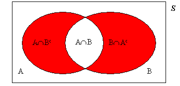
To see that P(Y = 1) = .7, note that the shaded areas below correspond
to this probability. 
Let D = "Defective". Let Y be a random variable and let it equal the number of the test on which the 2nd defective is found. Clearly
P(Y = 2) = P(D on draw 1)* P(D on draw 2) = 1/2 * 1/3 = 1/6
P(Y = 3) = P(D on draw 1) * P(Dc on draw 2) * P(D on draw 3) + P(Dc on draw 2) * P(D on draw 1) * P(D on draw 3)
Hence: P(Y = 2) = 1/2*2/3*1/2 + 1/2*2/3*1/2 = 2/6
Using similar reasoning:
P(Y = 4) = 1/2*2/3*1/2*1 + 1/2*2/3*1/2*1 + 1/2*1/3*1*1 = 3/6
                         æ  1/6  y = 2
                         ç
                         ç  2/6  y = 3
                  f(y) = ç
                         ç  3/6  y = 4
                         ç
                         è   0 otherwise