LEGACY CONTENT. If you are looking for Voteview.com, PLEASE CLICK HERE

This site is an archived version of Voteview.com archived from University of Georgia on May 23, 2017. This point-in-time capture includes all files publicly linked on Voteview.com at that time. We provide access to this content as a service to ensure that past users of Voteview.com have access to historical files. This content will remain online until at least January 1st, 2018. UCLA provides no warranty or guarantee of access to these files.

45-733 PROBABILITY AND STATISTICS I Notes #4D


February 2000


Conditional Distributions

  1. Recall that: P(A|B) = P(A Ç B)/P(B)
    The counterpart to this for distributions is:
    g1(x|y) = f(x,y)/f2(y) , where f2(y) > 0, the conditional distribution of x given y;
    and
    g2(y|x) = f(x,y)/f1(x) , where f1(x) > 0, the conditional distribution of y given x.

  2. These are legal probability distributions. To see this:
    ò-¥+¥ g1(x|y)dx = ò-¥+¥ [f(x,y)/f2(y)]dx =
    [1/f2(y)] [ò-¥+¥ f(x,y)dx] = [1/f2(y)][f2(y)] = 1

  3. Note that, with respect to f(x,y), conditional distributions are one-variable distributions because the value of one variable has been specified.
  4. If X and Y are Independent, then g1(x|y) = f1(x) and g2(y|x) = f2(y).

    To see this: g1(x|y) = f(x,y)/f2(y) = [f1(x)f2(y)]/f2(y) = f1(x).

  5. Example:
    
                               æ (1/12)(x - 2y)
                               ç         x = 2,3,4
                      f(x,y) = ç         y = 0,1
                               ç
                               è 0 otherwise


    Which yields the table:
    
                                   y
                               0       1
                             ------------
                           2 | 2       0 | 2
                             |           |
                        x  3 | 3       1 | 4
                             |           |
                           4 | 4       2 | 6
                             |           |
                             ---------------
                               9       3 |12
    

    To get g2(y|x=4) = f(4,y)/f1(4) =
    
                      æ 4/6 y = 0   because f(4,0)/f1(4) = (4/12)/(6/12)
                      ç                              
            g2(y|4) = ç 2/6 y = 1   because f(4,1)/f1(4) = (2/12)/(6/12)
                      ç                                  
                      è  0 otherwise
    

    To get g1(x|y=1) = f(x,1)/f2(1) =
    
                           æ  0  x = 2 
                           ç                              
                           ç 1/3 x = 3 
                 g1(x|1) = ç                                  
                           ç 2/3 x = 4                                  
                           ç                                  
                           è  0 otherwise
    

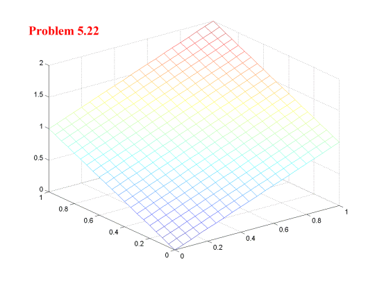
  6. Problem 5.22 p.208
    
                                æ y1 + y2
                                ç        0 < y1 < 1
                     f(y1,y2) = ç        0 < y2 < 1
                                ç
                                è  0 otherwise


    1. f1(y1) = ò01 f(y1, y2)dy2 = ò01 (y1 + y2)dy2 = [y1y2 + (y2)2)/2]|10 =
      y1 + 1/2
      Hence:
      
                æ y1 + 1/2                    æ y2 + 1/2
                ç                             ç
       f1(y1) = ç       0 < y1 < 1    f2(y2) = ç        0 < y2 < 1
                ç                             ç
                è  0 otherwise                è  0 otherwise
      

    2. P[Y1 ³ 1/2 | Y2 ³ 1/2] = P[Y1 ³ 1/2 Ç Y2 ³ 1/2]/P[Y2 ³ 1/2]
      Working the Numerator first:
      ò1/21 ò1/21 (y1 + y2)dy1dy2 = ò1/21 [(y1)2)/2 + y1y2]|11/2 dy2 =
      ò1/21 [1/2 + y2 - 1/8 - (y2)/2]dy2 = ò1/21 [3/8 + (y2)/2]dy2 =
      [(3/8)y2 + (y2)2)/2]|11/2 = 3/8
      To get the Denominator we can use the marginal distribution from (a):
      P(Y2 ³ 1/2) = ò1/21 [y2 + 1/2]dy2 = [(y2)2)/2 + (1/2)y2]| 11/2 = 5/8
      Hence, the answer is (3/8)/(5/8) = 3/5


    3. Solve: P[Y1 ³ 1/2 | Y2 = 1/2]
      Note that, although this looks like:
      P[Y1 ³ 1/2 | Y2 ³ 1/2]
      it is very different! Here we are only dealing with one variable whereas in (b) we were dealing with two variables. In part (b) the answer was the ratio of two volumes. Here the answer is the area under a curve which is a slice through the bivariate distribution.
      To solve this problem we need g1(y1|y2 = 1/2)
      In this case, we can use (a) to get:
      g1(y1|y2 = 1/2) = f(y1, y2)/f2(y2) = (y1+ y2)/(y2 + 1/2) = (y1+ 1/2)/(1/2 + 1/2) = y1+ 1/2
      Hence:
      
                              æ y1 + 1/2
                              ç        0 < y1 < 1
               g(y1|y2=1/2) = ç        
                              ç
                              è  0 otherwise
      

      Hence:
      ò3/41 [y1 + 1/2]dy1 = [(y1)2)/2 + y1/2]| 13/4 = 11/32
Covariance and Correlation

  1. Definition: Covariance
    COV(X,Y) = E{[X - E(X)][Y - E(Y)]} = E[XY - YE(X) - XE(Y) + E(X)E(Y)] =
    E(XY) - E(Y)E(X) - E(X)E(Y) + E(X)E(Y) = E(XY) - E(X)E(Y)

  2. If X and Y are Independent, then COV(X,Y) = 0
    (See (2) above.)

  3. Definition: Correlation
    
                       ______________
    r(X,Y) = COV(X,Y)/Ö[VAR(X)VAR(Y)]
    

  4. Correlation is just a standardized measure of covariance and it ranges from -1 to +1. A perfect positive correlation is +1 and a perfect negative correlation is -1.

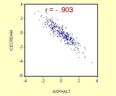
  5. It is important not to confuse correlation with causation. That two (or more) variables are correlated does not imply that one variable causes another! For example, viscosity of asphalt and consumption of ice cream are very highly negatively correlated. But we do not believe that consumption of ice cream causes asphalt to get softer! Rather, we know from the real world that it is the sun that causes both.


    Next mini in Stat II you will be faced with this issue a lot. It arises when you have to write down a model that expresses your belief about the relationship between different variables and then statistically test and interpret the results.

  6. Example: Compute COV(X,Y) and r(X,Y) for the bivariate discrete probability distribution in (10) above.
    1. COV(X,Y)
      E(XY) = åi=1,3 åj=1,2 xiyjf(xiyj) =
      2x0x2/12 + 2x1x0 + 3x0x3/12 + 3x1x1/12 + 4x0x4/12 + 4x1x2/12 = 11/12

      E(X) = åi=1,3 xif(xi) =
      2x2/12 + 3x4/12 + 4x6/12 = 40/12

      E(Y) = åj=1,2 yjf(yj) =
      0x9/12 + 1x3/12 = 3/12

      Hence, COV(X,Y) = 11/12 - (40/12)(3/12) = 12/144 = 1/12

    2. r(X,Y)
      E(X2) = åi=1,3 (xi)2f(xi) =
      4x2/12 + 9x4/12 + 16x6/12 = 140/12

      E(Y2) = åj=1,2 (yj)2f(yj) =
      0x9/12 + 1x3/12 = 3/12

      VAR(X) = 140/12 - (40/12)2 = 80/144
      VAR(Y) = 3/12 - (3/12)2 = 27/144

      Hence, r(X,Y)
      = (12/144)/[(80/144)(27/144)]1/2 = .258
  7. Recall that: If X1, X2, ... , Xn, are independent random variables, then:
    VAR(a1X1 + a2X2 + ... + anXn + b) = åi=1,n (ai)2VAR(Xi) = åi=1,n (ai)2 si2


  8. Dropping the assumption of Independence, this becomes:
    VAR(a1X1 + a2X2 + ... + anXn + b) = åi=1,n (ai)2VAR(Xi) +
    2[åi=1,n-1 åj=i+1,n aiajCOV(XiXj)]

    Note that åi=1,n-1 åj=i+1,n = (n choose 2).
  9. Example: Given
    VAR(X1) = 2 VAR(X2) = 4 VAR(X3) = 8
    COV(X1X2) = 1 COV(X1X3) = -1 COV(X1X2) = 2

    Find VAR(X1 + X2 + X3) = 2 + 4 + 8 + 2 - 2 + 4 = 18
    Find VAR(3X1 - X2 - 2X3 + 1) = 18 + 4 + 32 - 6 + 12 + 8 = 68
    Find VAR(X1 + 2X2 + 2X3 + 100) = 2 + 16 + 32 + 4 - 4 + 16 = 66