-
The first example is data generated from an MA(2).
IDENT(5) Y1
                      Correlogram of Y1
==============================================================
Date: 04/18/98   Time: 16:39
Sample: 1 100
Included observations: 99
==============================================================
 Autocorrelation Partial Correlation  AC     PAC  Q-Stat Prob
==============================================================
      . |**     |      . |**     |  1 0.293 0.293 8.7529 0.003
      .*| .     |      **| .     |  2-0.183-0.294 12.192 0.002
      .*| .     |      . |*.     |  3-0.084 0.085 12.929 0.005
      .*| .     |      .*| .     |  4-0.069-0.144 13.425 0.009
      .*| .     |      . | .     |  5-0.088-0.028 14.245 0.014
==============================================================
The Q-statistic is distributed as a
c2
distribution with 5 degrees of freedom
(5-0-0). Given that the p-value is 0.014 at lag 5, we reject the null hypothesis that
Y1 is white noise. First, try an MA(1) model:
LS Y1 C MA(1)
============================================================
LS // Dependent Variable is Y1
Date: 04/18/98   Time: 17:07
Sample(adjusted): 2 100
Included observations: 99 after adjusting endpoints
Convergence achieved after 8 iterations
============================================================
      Variable      CoefficienStd. Errort-Statistic  Prob.
============================================================
         C          -0.142594   0.156414  -0.911646   0.3642
       MA(1)         0.542028   0.085869   6.312245   0.0000
============================================================
R-squared            0.163421    Mean dependent var-0.140707
Adjusted R-squared   0.154796    S.D. dependent var 1.100216
S.E. of regression   1.011483    Akaike info criter 0.042831
Sum squared resid    99.24053    Schwarz criterion  0.095257
Log likelihood      -140.5950    F-statistic        18.94835
Durbin-Watson stat   2.174610    Prob(F-statistic)  0.000033
============================================================
Inverted MA Roots         -.54
============================================================
                   Correlogram of Residuals
==============================================================
Date: 04/18/98   Time: 17:08
Sample: 2 100
Included observations: 99
Q-statistic probabilities adjusted for 1 ARMA term(s)
==============================================================
 Autocorrelation Partial Correlation  AC     PAC  Q-Stat Prob
==============================================================
      .*| .     |      .*| .     |  1-0.094-0.094 0.8922
      .*| .     |      .*| .     |  2-0.133-0.143 2.7157 0.099
      . | .     |      . | .     |  3 0.014-0.014 2.7354 0.255
      .*| .     |      .*| .     |  4-0.072-0.094 3.2827 0.350
      . | .     |      . | .     |  5 0.008-0.010 3.2890 0.511
==============================================================
The P-Value for the 2nd lag is below .1 so it is a good idea to
check if adding an MA(2) term has an effect.LS Y1 C MA(1) MA(2)
============================================================
LS // Dependent Variable is Y1
Date: 04/18/98   Time: 17:11
Sample(adjusted): 2 100
Included observations: 99 after adjusting endpoints
Convergence achieved after 7 iterations
============================================================
      Variable      CoefficienStd. Errort-Statistic  Prob.
============================================================
         C          -0.142608   0.123090  -1.158568   0.2495
       MA(1)         0.429426   0.100236   4.284151   0.0000
       MA(2)        -0.204504   0.100171  -2.041551   0.0439
============================================================
R-squared            0.190999    Mean dependent var-0.140707
Adjusted R-squared   0.174144    S.D. dependent var 1.100216
S.E. of regression   0.999839    Akaike info criter 0.029512
Sum squared resid    95.96905    Schwarz criterion  0.108152
Log likelihood      -138.9358    F-statistic        11.33240
Durbin-Watson stat   1.967454    Prob(F-statistic)  0.000038
============================================================
Inverted MA Roots          .2      -.72
============================================================
The MA(2) coefficient is statistically significant and the correlogram
of the residuals below indicates that the residuals are now white noise.
                   Correlogram of Residuals
==============================================================
Date: 04/18/98   Time: 17:12
Sample: 2 100
Included observations: 99
Q-statistic probabilities adjusted for 2 ARMA term(s)
==============================================================
 Autocorrelation Partial Correlation  AC     PAC  Q-Stat Prob
==============================================================
      . | .     |      . | .     |  1 0.008 0.008 0.0073
      . | .     |      . | .     |  2-0.009-0.009 0.0151
      .*| .     |      .*| .     |  3-0.068-0.068 0.4946 0.482
      .*| .     |      .*| .     |  4-0.059-0.058 0.8553 0.652
      .*| .     |      .*| .     |  5-0.059-0.060 1.2260 0.747
==============================================================
In this second example, the series was generated from a MA(4)
process.IDENT Y2
                      Correlogram of Y2
==============================================================
Date: 04/18/98   Time: 17:16
Sample: 1 100
Included observations: 96
==============================================================
 Autocorrelation Partial Correlation  AC     PAC  Q-Stat Prob
==============================================================
      . |***    |      . |***    |  1 0.374 0.374 13.839 0.000
      . |**     |      . |*.     |  2 0.210 0.081 18.243 0.000
      . | .     |      .*| .     |  3-0.018-0.141 18.275 0.000
     ***| .     |     ***| .     |  4-0.402-0.442 34.800 0.000
      .*| .     |      . |**     |  5-0.111 0.255 36.072 0.000
==============================================================
There are spikes at 1, 2, and 4 which indicates that we could start with the
corresponding model:LS Y2 C MA(1) MA(2) MA(4)
============================================================
LS // Dependent Variable is Y2
Date: 04/18/98   Time: 17:18
Sample(adjusted): 5 100
Included observations: 96 after adjusting endpoints
Convergence achieved after 23 iterations
============================================================
      Variable      CoefficienStd. Errort-Statistic  Prob.
============================================================
         C          -0.247163   0.088734  -2.785441   0.0065
       MA(1)         0.270512   0.014926   18.12332   0.0000
       MA(2)         0.241476   0.023006   10.49631   0.0000
       MA(4)        -0.741378   0.000426  -1741.355   0.0000
============================================================
R-squared            0.430208    Mean dependent var-0.249292
Adjusted R-squared   0.411628    S.D. dependent var 1.437408
S.E. of regression   1.102570    Akaike info criter 0.236061
Sum squared resid    111.8408    Schwarz criterion  0.342909
Log likelihood      -143.5490    F-statistic        23.15415
Durbin-Watson stat   1.583374    Prob(F-statistic)  0.000000
============================================================
Inverted MA Roots          .8  -.08 -.99  -.08+.99i      -.93
============================================================
Given the low P-Values at several of the lags, we reject the
null hypothesis that we have white noise. Given the small spike
at the 3rd lag -- the term we did not estimate -- this
is what we should try next.
                   Correlogram of Residuals
==============================================================
Date: 04/18/98   Time: 17:19
Sample: 5 100
Included observations: 96
Q-statistic probabilities adjusted for 3 ARMA term(s)
==============================================================
 Autocorrelation Partial Correlation  AC     PAC  Q-Stat Prob
==============================================================
      . |**     |      . |**     |  1 0.203 0.203 4.0771
      . |*.     |      . |*.     |  2 0.126 0.088 5.6644
      . |*.     |      . |*.     |  3 0.114 0.077 6.9852
      . | .     |      . | .     |  4 0.026-0.020 7.0561 0.008
      . | .     |      . | .     |  5-0.025-0.047 7.1193 0.028
      .*| .     |      .*| .     |  6-0.116-0.119 8.5215 0.036
      . | .     |      . | .     |  7-0.022 0.027 8.5709 0.073
      . |*.     |      . |*.     |  8 0.098 0.137 9.6070 0.087
      .*| .     |      .*| .     |  9-0.065-0.088 10.063 0.122
      . | .     |      . | .     | 10 0.029 0.035 10.154 0.180
==============================================================
LS Y2 C MA(1) MA(2) MA(3) MA(4)
============================================================
LS // Dependent Variable is Y2
Date: 04/18/98   Time: 17:23
Sample(adjusted): 5 100
Included observations: 96 after adjusting endpoints
Convergence achieved after 14 iterations
============================================================
      Variable      CoefficienStd. Errort-Statistic  Prob.
============================================================
         C          -0.241779   0.141800  -1.705070   0.0916
       MA(1)         0.417588   0.033201   12.57753   0.0000
       MA(2)         0.347918   0.024563   14.16449   0.0000
       MA(3)         0.177436   0.034332   5.168260   0.0000
       MA(4)        -0.657530   0.000420  -1564.053   0.0000
============================================================
R-squared            0.451218    Mean dependent var-0.249292
Adjusted R-squared   0.427095    S.D. dependent var 1.437408
S.E. of regression   1.087981    Akaike info criter 0.219325
Sum squared resid    107.7169    Schwarz criterion  0.352885
Log likelihood      -141.7457    F-statistic        18.70542
Durbin-Watson stat   1.895751    Prob(F-statistic)  0.000000
============================================================
Inverted MA Roots          .6  -.07+.99i  -.07 -.99      -.97
============================================================
All the MA terms are statistically significant and the P-Values of the correlogram
indicate that we have white noise.
                   Correlogram of Residuals
==============================================================
Date: 04/18/98   Time: 17:24
Sample: 5 100
Included observations: 96
Q-statistic probabilities adjusted for 4 ARMA term(s)
==============================================================
 Autocorrelation Partial Correlation  AC     PAC  Q-Stat Prob
==============================================================
      . | .     |      . | .     |  1 0.048 0.048 0.2327
      . | .     |      . | .     |  2 0.049 0.047 0.4779
      . | .     |      . | .     |  3 0.012 0.007 0.4920
      . | .     |      . | .     |  4 0.001-0.002 0.4921
      .*| .     |      .*| .     |  5-0.083-0.084 1.1997 0.273
      .*| .     |      .*| .     |  6-0.131-0.125 2.9944 0.224
      .*| .     |      . | .     |  7-0.066-0.049 3.4496 0.327
      . |*.     |      . |*.     |  8 0.121 0.143 5.0195 0.285
      .*| .     |      .*| .     |  9-0.092-0.096 5.9386 0.312
      . | .     |      . | .     | 10 0.035 0.027 6.0755 0.415
==============================================================
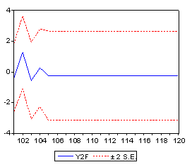
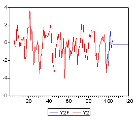
To forecast this series issue the following commands (see Epple Notes
XIII-13):EXPAND 120
SMPL 1 120
Then go into the "Forecast" menu (click the button). In the forecast menu enter a name for the standard error series and click the plot button. You will see:

PLOT Y2F Y2
