1998 Flex-Time and Flex-Mode Prob-Stat II ARIMA (Part 2) Page
LEGACY CONTENT.
If you are looking for Voteview.com, PLEASE CLICK HEREThis site is an archived version of Voteview.com archived from University of Georgia on
May 23, 2017. This point-in-time capture includes all files publicly linked on Voteview.com at that time. We provide access to this content as a service to ensure that past users of Voteview.com have access to historical files. This content will remain online until at least
January 1st, 2018. UCLA provides no warranty or guarantee of access to these files.
45-734 PROBABILITY AND STATISTICS II (4th Mini AY1997-98)
ARIMA Examples (Part 2)
Nonstationary series can usually be converted into stationary series by
simple differencing; that is:
Dyt = yt - yt-1
Sometimes, after differencing, the resulting series is still not
stationary. If so, the series can be differenced again:
D2yt =
Dyt -
Dyt-1
Another common form of differencing is to take the difference of the
logs; that is:
Lyt = ln(yt) - ln(yt-1)
Once a stationary series is obtained, we can proceed to estimate AR(.)
and MA(.) terms just as before and we can generate forecasts.
Example 1:
A telltale sign of a nonstationary series is a spike at lag 1 in the
PACF coupled with an ACF that trails off very slowly.
IDENT(5) YY5
                      Correlogram of YY5
==============================================================
Date: 04/28/98   Time: 14:07
Sample: 1 100
Included observations: 100
==============================================================
 Autocorrelation Partial Correlation  AC     PAC  Q-Stat Prob
==============================================================
      . |*******|      . |*******|  1 0.960 0.960 94.948 0.000
      . |*******|      .*| .     |  2 0.916-0.069 182.30 0.000
      . |*******|      . | .     |  3 0.875 0.014 262.81 0.000
      . |****** |      . | .     |  4 0.834-0.025 336.69 0.000
      . |****** |      . | .     |  5 0.790-0.055 403.72 0.000
==============================================================
This pattern indicates a nonstationary series. Taking the first
differences the Correlogram is:
                  Correlogram of YY5-YY5(-1)
==============================================================
Date: 04/28/98   Time: 14:09
Sample: 1 100
Included observations: 99
==============================================================
 Autocorrelation Partial Correlation  AC     PAC  Q-Stat Prob
==============================================================
      . |***    |      . |***    |  1 0.394 0.394 15.823 0.000
      .*| .     |      **| .     |  2-0.059-0.254 16.185 0.000
      . |*.     |      . |**     |  3 0.120 0.316 17.692 0.001
      . | .     |      **| .     |  4 0.023-0.274 17.747 0.001
      .*| .     |      . |*.     |  5-0.065 0.180 18.190 0.003
==============================================================
The series now appears to be stationary. The spikes at one lag in the
ACF and PACF indicate that we should first try a simple MA(1) model. (Note
that we can use the D(.) operator built into EVIEWS to do the first
differencing; that is:
D(YY5) = YY5-YY5(-1), so that:
LS D(YY5) C MA(1)
============================================================
LS // Dependent Variable is D(YY5)
Date: 04/28/98   Time: 14:58
Sample(adjusted): 2 100
Included observations: 99 after adjusting endpoints
Convergence achieved after 7 iterations
============================================================
      Variable      CoefficienStd. Errort-Statistic  Prob.
============================================================
         C           0.504227   0.188794   2.670780   0.0089
       MA(1)         0.801583   0.060328   13.28703   0.0000
============================================================
R-squared            0.343359    Mean dependent var 0.500937
Adjusted R-squared   0.336589    S.D. dependent var 1.281686
S.E. of regression   1.043934    Akaike info criter 0.105987
Sum squared resid    105.7104    Schwarz criterion  0.158414
Log likelihood      -143.7213    F-statistic        50.72140
Durbin-Watson stat   2.146790    Prob(F-statistic)  0.000000
============================================================
Inverted MA Roots         -.80
============================================================
The Correlogram of the residuals is:
                   Correlogram of Residuals
==============================================================
Date: 04/28/98   Time: 14:12
Sample: 2 100
Included observations: 99
Q-statistic probabilities adjusted for 1 ARMA term(s)
==============================================================
 Autocorrelation Partial Correlation  AC     PAC  Q-Stat Prob
==============================================================
      .*| .     |      .*| .     |  1-0.074-0.074 0.5595
      .*| .     |      .*| .     |  2-0.094-0.100 1.4615 0.227
      . |*.     |      . |*.     |  3 0.153 0.140 3.8927 0.143
      . | .     |      . | .     |  4 0.003 0.016 3.8934 0.273
      .*| .     |      .*| .     |  5-0.120-0.096 5.4250 0.246
==============================================================
The p-values are all large so we cannot reject the null hypothesis
that the residuals are white noise.
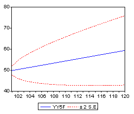
To forecast the series we first expand the series:
EXPAND 120
Then we go into the "Forecast" button and enter 101 120 in the
"Sample Range for Forecast", click the button for graph, and enter
a name for the standard error series. Click OK and you get:

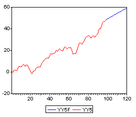
Now to see the whole series plus the forecast type:
PLOT YY5F YY5

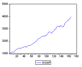
Real GNP from 1947 (1) to 1988 (3):
It is clear from the plot of real GNP that it is not a stationary time series.

Note the pattern below of the ACFs and PACFs:
                     Correlogram of RGNP
==============================================================
Date: 04/28/98   Time: 15:46
Sample: 1 180
Included observations: 167
==============================================================
 Autocorrelation Partial Correlation  AC     PAC  Q-Stat Prob
==============================================================
       .|********       .|********  1 0.980 0.980 163.34 0.000
       .|*******|       .|.      |  2 0.960-0.018 320.97 0.000
       .|*******|       .|.      |  3 0.940-0.015 472.91 0.000
       .|*******|       .|.      |  4 0.919-0.007 619.26 0.000
       .|*******|       .|.      |  5 0.900 0.002 760.25 0.000
==============================================================
The appropriate fixup here is to take the first difference of the logs
of real GNP. You can do this by using the DLOG(.) command in EVIEWS
which computes the first difference in the natural logs. That is:
DLOG(RGNP) = LOG(RGNP) - LOG(RGNP(-1))
                  Correlogram of DLOG(RGNP)
==============================================================
Date: 04/28/98   Time: 15:51
Sample: 1 180
Included observations: 166
==============================================================
 Autocorrelation Partial Correlation  AC     PAC  Q-Stat Prob
==============================================================
       .|***    |       .|***    |  1 0.370 0.370 23.170 0.000
       .|**     |       .|*      |  2 0.249 0.130 33.743 0.000
       .|.      |       *|.      |  3 0.000-0.151 33.743 0.000
       *|.      |       *|.      |  4-0.102-0.109 35.525 0.000
       *|.      |       .|.      |  5-0.117-0.019 37.899 0.000
==============================================================
The ACFs and PACFs and the graph of the transformed time series offer
solid evidence that we have a stationary time series. The spikes in the
first lag indicates that we should try a MA(1) model first.
LS DLOG(RGNP) C MA(1)
============================================================
LS // Dependent Variable is DLOG(RGNP)
Date: 04/28/98   Time: 15:55
Sample(adjusted): 2 167
Included observations: 166 after adjusting endpoints
Convergence achieved after 10 iterations
============================================================
      Variable      CoefficienStd. Errort-Statistic  Prob.
============================================================
         C           0.008031   0.001019   7.877449   0.0000
       MA(1)         0.268213   0.075216   3.565924   0.0005
============================================================
R-squared            0.098695    Mean dependent var 0.008034
Adjusted R-squared   0.093200    S.D. dependent var 0.010885
S.E. of regression   0.010365    Akaike info criter-9.126620
Sum squared resid    0.017620    Schwarz criterion -9.089126
Log likelihood       523.9656    F-statistic        17.95845
Durbin-Watson stat   1.859536    Prob(F-statistic)  0.000038
============================================================
Inverted MA Roots         -.27
============================================================
                   Correlogram of Residuals
==============================================================
Date: 04/28/98   Time: 15:55
Sample: 2 167
Included observations: 166
Q-statistic probabilities adjusted for 1 ARMA term(s)
==============================================================
 Autocorrelation Partial Correlation  AC     PAC  Q-Stat Prob
==============================================================
       .|*      |       .|*      |  1 0.070 0.070 0.8294
       .|**     |       .|**     |  2 0.252 0.248 11.613 0.001
       .|.      |       *|.      |  3-0.045-0.081 11.958 0.003
       *|.      |       *|.      |  4-0.071-0.135 12.823 0.005
       *|.      |       .|.      |  5-0.093-0.054 14.335 0.006
==============================================================
The spike at the second lag of the ACF and PACF suggests adding a
MA(2) term to the model.
LS DLOG(RGNP) C MA(1) MA(2)
============================================================
LS // Dependent Variable is DLOG(RGNP)
Date: 04/28/98   Time: 15:57
Sample(adjusted): 2 167
Included observations: 166 after adjusting endpoints
Convergence achieved after 7 iterations
============================================================
      Variable      CoefficienStd. Errort-Statistic  Prob.
============================================================
         C           0.008027   0.001224   6.557310   0.0000
       MA(1)         0.304527   0.075294   4.044511   0.0001
       MA(2)         0.274132   0.075290   3.641029   0.0004
============================================================
R-squared            0.165012    Mean dependent var 0.008034
Adjusted R-squared   0.154767    S.D. dependent var 0.010885
S.E. of regression   0.010007    Akaike info criter-9.190997
Sum squared resid    0.016323    Schwarz criterion -9.134756
Log likelihood       530.3090    F-statistic        16.10617
Durbin-Watson stat   1.949344    Prob(F-statistic)  0.000000
============================================================
Inverted MA Roots     -.15 -.  -.15+.50i
============================================================


                   Correlogram of Residuals
==============================================================
Date: 04/28/98   Time: 15:57
Sample: 2 167
Included observations: 166
Q-statistic probabilities adjusted for 2 ARMA term(s)
==============================================================
 Autocorrelation Partial Correlation  AC     PAC  Q-Stat Prob
==============================================================
       .|.      |       .|.      |  1 0.025 0.025 0.1079
       .|.      |       .|.      |  2 0.018 0.017 0.1626
       .|.      |       .|.      |  3 0.044 0.043 0.4910 0.483
       *|.      |       *|.      |  4-0.084-0.087 1.7072 0.426
       *|.      |       *|.      |  5-0.116-0.114 4.0405 0.257
==============================================================
The p-values are quite large so we do not reject the null hypothesis
that we have white noise. This appears to be the correct model.
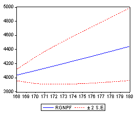
To forecast Real GNP through 1991 first expand the series and change the
sample range:
EXPAND 180
SMPL 168 180
Now go to the "Forecast" window and make up a name for the standard error
series. Clicking "OK" produces the following plot:

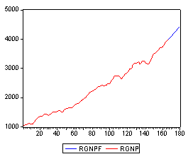
To look at the original series and the forecast issue the commands:
SMPL 1 180
PLOT RGNPF RGNP
