1998 Flex-Time and Flex-Mode Prob-Stat II Note Set 6 Handouts Page
LEGACY CONTENT.
If you are looking for Voteview.com, PLEASE CLICK HEREThis site is an archived version of Voteview.com archived from University of Georgia on
May 23, 2017. This point-in-time capture includes all files publicly linked on Voteview.com at that time. We provide access to this content as a service to ensure that past users of Voteview.com have access to historical files. This content will remain online until at least
January 1st, 2018. UCLA provides no warranty or guarantee of access to these files.
45-734 PROBABILITY AND STATISTICS II (4th Mini AY1997-98)
Note Set 6 Handouts
KEPLER.WF1 Examples
LS DAYS C DIST
HIST RESID

Note that the Probability here is 0.668929 so we do not reject the null
hypothesis that residuals are normally distributed.
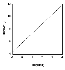
SCAT(R) LOG(DAYS) LOG(DIST)

LS LOG(DAYS) C LOG(DIST)
============================================================
LS // Dependent Variable is LOG(DAYS)
Date: 04/04/98   Time: 17:18
Sample: 1 9
Included observations: 9
============================================================
      Variable      CoefficienStd. Errort-Statistic  Prob.
============================================================
         C           5.901252   0.001346   4385.273   0.0000
     LOG(DIST)       1.498890   0.000617   2430.848   0.0000
============================================================
R-squared            0.999999    Mean dependent var 8.081784
Adjusted R-squared   0.999999    S.D. dependent var 2.586347
S.E. of regression   0.003009    Akaike info criter-11.41893
Sum squared resid    6.34E-05    Schwarz criterion -11.37510
Log likelihood       40.61473    F-statistic        5909021.
Durbin-Watson stat   1.598728    Prob(F-statistic)  0.000000
============================================================
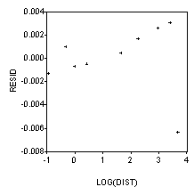
SCAT RESID LOG(DIST)

Note the scale on the residuals!
To directly test Kepler's 3rd Law:
LS DAYS^2 C DIST^3
============================================================
LS // Dependent Variable is DAYS^2
Date: 04/04/98   Time: 17:27
Sample: 1 9
Included observations: 9
============================================================
      Variable      CoefficienStd. Errort-Statistic  Prob.
============================================================
         C           7012275.   9104212.   0.770223   0.4664
       DIST^3        131103.7   396.1369   330.9556   0.0000
============================================================
R-squared            0.999936    Mean dependent var 1.44E+09
Adjusted R-squared   0.999927    S.D. dependent var 2.81E+09
S.E. of regression   24038144    Akaike info criter 34.18343
Sum squared resid    4.04E+15    Schwarz criterion  34.22726
Log likelihood      -164.5959    F-statistic        109531.6
Durbin-Watson stat   2.174360    Prob(F-statistic)  0.000000
============================================================
WINDMILL.WF1 Examples
LS DCOUT C WIND
============================================================
LS // Dependent Variable is DCOUT
Date: 04/04/98   Time: 17:30
Sample: 1 25
Included observations: 25
============================================================
      Variable      CoefficienStd. Errort-Statistic  Prob.
============================================================
         C           0.130875   0.125989   1.038779   0.3097
        WIND         0.241149   0.019049   12.65927   0.0000
============================================================
R-squared            0.874493    Mean dependent var 1.609600
Adjusted R-squared   0.869036    S.D. dependent var 0.652278
S.E. of regression   0.236052    Akaike info criter-2.810787
Sum squared resid    1.281573    Schwarz criterion -2.713277
Log likelihood       1.661381    F-statistic        160.2571
Durbin-Watson stat   0.536610    Prob(F-statistic)  0.000000
============================================================
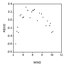
SCAT RESID WIND

Ramsey Reset Test With One Fitted Term. Note that we reject
the null hypothesis that we have a linear specification (that is, the
y-hat-squared variable is statistically significant).
============================================================
Ramsey RESET Test:
============================================================
F-statistic          63.16035    Probability        0.000000
Log likelihood ratio 33.83734    Probability        0.000000
============================================================

Test Equation:
LS // Dependent Variable is DCOUT
Date: 04/04/98   Time: 17:33
Sample: 1 25
Included observations: 25
============================================================
      Variable      CoefficienStd. Errort-Statistic  Prob.
============================================================
         C          -1.144670   0.173341  -6.603572   0.0000
        WIND         0.764313   0.066569   11.48152   0.0000
      Fitted^2      -0.655530   0.082484  -7.947349   0.0000
============================================================
R-squared            0.967577    Mean dependent var 1.609600
Adjusted R-squared   0.964630    S.D. dependent var 0.652278
S.E. of regression   0.122674    Akaike info criter-4.084281
Sum squared resid    0.331077    Schwarz criterion -3.938016
Log likelihood       18.58005    F-statistic        328.2660
Durbin-Watson stat   1.633283    Prob(F-statistic)  0.000000
============================================================
Ramsey Reset Test With Three Fitted Terms. Note that we reject
the null hypothesis that we have a linear specification (that is, the
(y-hat)2, (y-hat)3, and (y-hat)4
variables are jointly significant!).
============================================================
Ramsey RESET Test:
============================================================
F-statistic          39.22341    Probability        0.000000
Log likelihood ratio 48.22822    Probability        0.000000
============================================================

Test Equation:
LS // Dependent Variable is DCOUT
Date: 04/04/98   Time: 17:37
Sample: 1 25
Included observations: 25
============================================================
      Variable      CoefficienStd. Errort-Statistic  Prob.
============================================================
         C          -4.499507   1.028285  -4.375738   0.0003
        WIND         4.052803   1.096749   3.695287   0.0014
      Fitted^2      -13.20964   4.522482  -2.920883   0.0085
      Fitted^3       4.820264   1.900918   2.535756   0.0197
      Fitted^4      -0.659612   0.286779  -2.300075   0.0323
============================================================
R-squared            0.981767    Mean dependent var 1.609600
Adjusted R-squared   0.978120    S.D. dependent var 0.652278
S.E. of regression   0.096483    Akaike info criter-4.499916
Sum squared resid    0.186180    Schwarz criterion -4.256141
Log likelihood       25.77549    F-statistic        269.2287
Durbin-Watson stat   2.511711    Prob(F-statistic)  0.000000
============================================================
LS DCOUT C WIND WIND^2 WIND^3
============================================================
LS // Dependent Variable is DCOUT
Date: 04/04/98   Time: 17:43
Sample: 1 25
Included observations: 25
============================================================
      Variable      CoefficienStd. Errort-Statistic  Prob.
============================================================
         C          -2.358550   0.438464  -5.379120   0.0000
        WIND         1.426866   0.246758   5.782440   0.0000
       WIND^2       -0.160366   0.042056  -3.813172   0.0010
       WIND^3        0.006458   0.002211   2.920922   0.0082
============================================================
R-squared            0.976944    Mean dependent var 1.609600
Adjusted R-squared   0.973650    S.D. dependent var 0.652278
S.E. of regression   0.105881    Akaike info criter-4.345226
Sum squared resid    0.235428    Schwarz criterion -4.150206
Log likelihood       22.84186    F-statistic        296.6100
Durbin-Watson stat   2.122609    Prob(F-statistic)  0.000000
============================================================
Here is the correct specification:
LS DCOUT C 1/WIND
============================================================
LS // Dependent Variable is DCOUT
Date: 04/04/98   Time: 17:45
Sample: 1 25
Included observations: 25
============================================================
      Variable      CoefficienStd. Errort-Statistic  Prob.
============================================================
         C           2.978860   0.044902   66.34096   0.0000
       1/WIND       -6.934547   0.206434  -33.59215   0.0000
============================================================
R-squared            0.980025    Mean dependent var 1.609600
Adjusted R-squared   0.979156    S.D. dependent var 0.652278
S.E. of regression   0.094171    Akaike info criter-4.648660
Sum squared resid    0.203970    Schwarz criterion -4.551150
Log likelihood       24.63479    F-statistic        1128.433
Durbin-Watson stat   2.269181    Prob(F-statistic)  0.000000
============================================================
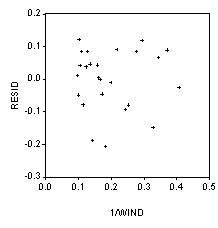
SCAT RESID 1/WIND

Ramsey Reset Test With One Fitted Term. Note that we do
not reject
the null hypothesis that we have a linear specification (that is, the
y-hat-squared variable is not statistically significant).
============================================================
Ramsey RESET Test:
============================================================
F-statistic          0.773032    Probability        0.388784
Log likelihood ratio 0.863364    Probability        0.352799
============================================================

Test Equation:
LS // Dependent Variable is DCOUT
Date: 04/04/98   Time: 17:49
Sample: 1 25
Included observations: 25
============================================================
      Variable      CoefficienStd. Errort-Statistic  Prob.
============================================================
         C           2.671045   0.352996   7.566788   0.0000
       1/WIND       -6.072507   1.002167  -6.059378   0.0000
      Fitted^2       0.046004   0.052323   0.879222   0.3888
============================================================
R-squared            0.980703    Mean dependent var 1.609600
Adjusted R-squared   0.978949    S.D. dependent var 0.652278
S.E. of regression   0.094639    Akaike info criter-4.603194
Sum squared resid    0.197046    Schwarz criterion -4.456929
Log likelihood       25.06647    F-statistic        559.0351
Durbin-Watson stat   2.400475    Prob(F-statistic)  0.000000
============================================================
MPG.WF1 Examples
LS MPG C SPEED SPEED^2
============================================================
LS // Dependent Variable is MPG
Date: 04/04/98   Time: 17:52
Sample: 1 12
Included observations: 12
============================================================
      Variable      CoefficienStd. Errort-Statistic  Prob.
============================================================
         C          -182.5821   17.67703  -10.32878   0.0000
       SPEED         8.983214   0.761563   11.79575   0.0000
      SPEED^2       -0.091071   0.007993  -11.39408   0.0000
============================================================
R-squared            0.947388    Mean dependent var 32.00000
Adjusted R-squared   0.935696    S.D. dependent var 6.809085
S.E. of regression   1.726658    Akaike info criter 1.304694
Sum squared resid    26.83214    Schwarz criterion  1.425921
Log likelihood      -21.85543    F-statistic        81.03174
Durbin-Watson stat   2.102570    Prob(F-statistic)  0.000002
============================================================
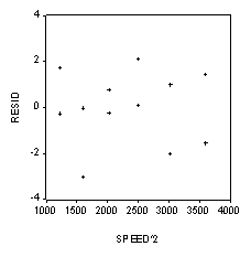
SCAT RESID SPEED^2

Under View select Representation
Estimation Command:
=====================
LS MPG C SPEED SPEED^2

Estimation Equation:
=====================
MPG = C(1) + C(2)*SPEED + C(3)*(SPEED^2)

Substituted Coefficients:
=====================
MPG = -182.58214 + 8.9832143*SPEED - 0.091071429*(SPEED^2)
Under View select Coefficient Test then select
Wald Test. Note that this is testing a null hypothesis
that the most efficient speed is 50 mph. We do not reject this
null hypothesis.
====================================================
Wald Test:
Equation: Untitled
====================================================
Null HypothesisC(3)=-C(2)/100
====================================================
F-statistic     3.068953    Probability     0.113713
Chi-square      3.068953    Probability     0.079801
====================================================

