1. (5 Points) Examine the three regressions below. What is the correlation between X1 and X2?
The correlation is approximately zero: COR(X1, X2) » 0.
============================================================
LS // Dependent Variable is Y
Date: 04/14/98   Time: 14:46
Sample: 1 2556
Included observations: 2556
============================================================
     Variable     Coefficient Std. ErrorT-Statistic  Prob.
============================================================
        C            1.993122   0.050877   39.29572   0.0000
        X1           2.000000   0.067508   31.04490   0.0000
        X2          -2.000000   0.068177  -30.15076   0.0000
============================================================
R-squared            0.419060    Mean dependent var 2.012497
Adjusted R-squared   0.418605    S.D. dependent var 1.294197
S.E. of regression   0.986816    Akaike info criter-0.025370
Sum squared resid    2486.128    Schwartz criterion-0.018508
Log likelihood      -3591.384    F-statistic        920.7998
Durbin-Watson stat   1.957578    Prob(F-statistic)  0.000000
============================================================

============================================================
LS // Dependent Variable is Y
Date: 04/14/98   Time: 14:46
Sample: 1 2556
Included observations: 2556
============================================================
     Variable     Coefficient Std. ErrorT-Statistic  Prob.
============================================================
        C            0.997764   0.044869   22.23732   0.0000
        X1           2.000000   0.078587   26.22855   0.0000
============================================================
R-squared            0.212199    Mean dependent var 2.012497
Adjusted R-squared   0.211891    S.D. dependent var 1.294197
S.E. of regression   1.148930    Akaike info criter 0.278445
Sum squared resid    3371.385    Schwartz criterion 0.283019
Log likelihood      -3980.659    F-statistic        687.9368
Durbin-Watson stat   1.950712    Prob(F-statistic)  0.000000
============================================================

============================================================
LS // Dependent Variable is Y
Date: 04/14/98   Time: 14:46
Sample: 1 2556
Included observations: 2556
============================================================
     Variable     Coefficient Std. ErrorT-Statistic  Prob.
============================================================
        C            3.013179   0.045775   65.82524   0.0000
        X2          -2.000000   0.079990  -25.24868   0.0000
============================================================
R-squared            0.199748    Mean dependent var 2.012497
Adjusted R-squared   0.199435    S.D. dependent var 1.294197
S.E. of regression   1.157974    Akaike info criter 0.294126
Sum squared resid    3424.669    Schwartz criterion 0.298701
Log likelihood      -4000.700    F-statistic        637.4959
Durbin-Watson stat   2.058143    Prob(F-statistic)  0.000000
============================================================
Probability and Statistics Name_________________________________
2. (10 Points) Consider the model of refrigerator price shown on page IV-13 of Epple Notes IV. Suppose we have obtain the following data on a new refrigerator: PRICE = $465, OPCOST = 69, REFRSIZE = 14.1, FREZSIZE = 4.5, SHELVES = 3, FEATURES = 4. Test whether or not this new refrigerator fits the same linear model as that shown for the current 37 refrigerators (report the relevant statistics).
Using the Chow Forecast Test we get:
F-statistic 6.452158 Probability 0.016310
This is a low P-Value, so we would reject the null hypothesis that this observation fits the same linear model as for the first 37 refrigerators.
Probability and Statistics Name_________________________________
3. (5 Points) Suppose you are analyzing some data and obtain the output shown below. Y and X are gathered over time. What should you do next (give the EVIEWS commands)?
LS Y C X AR(1)
Then look at the Durban-Watson to see it is near 2.0. If not, add AR(2); etc.
============================================================
LS // Dependent Variable is Y
Date: 04/15/98   Time: 15:21
Sample: 1 50
Included observations: 50
============================================================
     Variable     Coefficient Std. ErrorT-Statistic  Prob.
============================================================
        C            1.919646   0.026538   72.33622   0.0000
        X            1.993785   0.025803   77.26945   0.0000
============================================================
R-squared            0.923012    Mean dependent var 1.979271
Adjusted R-squared   0.922858    S.D. dependent var 2.135603
S.E. of regression   0.593153    Akaike info criter-1.040614
Sum squared resid    175.2116    Schwartz criterion-1.023755
Log likelihood      -447.3158    F-statistic        5970.568
Durbin-Watson stat   0.937929    Prob(F-statistic)  0.000000
============================================================
Probability and Statistics Name_________________________________
4. (10 Points) Analyze the four regressions below. What do you think accounts for the pattern of coefficients and p-values in the four regressions? What would you do next? Give the relevant EVIEWS commands.
Multicollinearity between X1, X2, and X3. The first thing to try is to look at the correlation matrix:
COR X1 X2 X3
Then a good thing to do would be to look at the scatterplots:
SCAT(R) X1 X2
Etc
Finally, regress each independent variable on the other two to see what is going on.
LS X1 C X2 X3,
LS X2 C X1 X3,
LS X3 C X1 X2
============================================================
LS // Dependent Variable is Y
Date: 04/15/98   Time: 15:39
Sample: 1 50
Included observations: 50
============================================================
     Variable     Coefficient Std. ErrorT-Statistic  Prob.
============================================================
        C            2.029421   0.147004   13.80522   0.0000
        X1           0.541664   1.351931   0.400659   0.6905
        X2           4.884678   2.062344   2.368508   0.0221
        X3           2.645894   0.670848   3.944103   0.0003
============================================================
R-squared            0.979241    Mean dependent var 1.650988
Adjusted R-squared   0.977888    S.D. dependent var 6.809458
S.E. of regression   1.012582    Akaike info criter 0.101625
Sum squared resid    47.16479    Schwartz criterion 0.254586
Log likelihood      -69.48754    F-statistic        723.3186
Durbin-Watson stat   1.683583    Prob(F-statistic)  0.000000
============================================================

============================================================
LS // Dependent Variable is Y
Date: 04/15/98   Time: 15:39
Sample: 1 50
Included observations: 50
============================================================
     Variable     Coefficient Std. ErrorT-Statistic  Prob.
============================================================
        C            1.917990   0.165098   11.61727   0.0000
        X1           5.845753   0.158529   36.87503   0.0000
        X2          -3.225081   0.182444  -17.67712   0.0000
============================================================
R-squared            0.972221    Mean dependent var 1.650988
Adjusted R-squared   0.971039    S.D. dependent var 6.809458
S.E. of regression   1.158820    Akaike info criter 0.352930
Sum squared resid    63.11463    Schwartz criterion 0.467651
Log likelihood      -76.77016    F-statistic        822.4778
Durbin-Watson stat   1.863547    Prob(F-statistic)  0.000000
============================================================
============================================================
LS // Dependent Variable is Y
Date: 04/15/98   Time: 15:40
Sample: 1 50
Included observations: 50
============================================================
     Variable     Coefficient Std. ErrorT-Statistic  Prob.
============================================================
        C            1.960444   0.150991   12.98382   0.0000
        X1           3.717884   0.179607   20.70011   0.0000
        X3           1.061739   0.054340   19.53864   0.0000
============================================================
R-squared            0.976710    Mean dependent var 1.650988
Adjusted R-squared   0.975719    S.D. dependent var 6.809458
S.E. of regression   1.061078    Akaike info criter 0.176695
Sum squared resid    52.91666    Schwartz criterion 0.291417
Log likelihood      -72.36431    F-statistic        985.5125
Durbin-Watson stat   1.812296    Prob(F-statistic)  0.000000
============================================================
============================================================
LS // Dependent Variable is Y
Date: 04/15/98   Time: 15:40
Sample: 1 50
Included observations: 50
============================================================
     Variable     Coefficient Std. ErrorT-Statistic  Prob.
============================================================
        C            2.040184   0.143232   14.24392   0.0000
        X2           5.704308   0.259119   22.01425   0.0000
        X3           2.913261   0.068121   42.76624   0.0000
============================================================
R-squared            0.979169    Mean dependent var 1.650988
Adjusted R-squared   0.978283    S.D. dependent var 6.809458
S.E. of regression   1.003498    Akaike info criter 0.065108
Sum squared resid    47.32938    Schwartz criterion 0.179830
Log likelihood      -69.57463    F-statistic        1104.627
Durbin-Watson stat   1.655416    Prob(F-statistic)  0.000000
============================================================
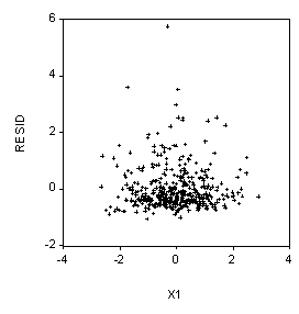
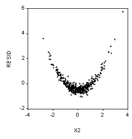
Probability and Statistics Name_________________________________5. (10 Points) Suppose our dependent variable is Y and we have two independent variables, X1 and X2. We use EVIEWS to run the regression:
LS Y C X1 X2
And then we produce the scatterplots below. What should we do next?
Try adding X2^2 to the model. That is, try:
LS Y C X1 X2 X2^2
Note that the Ramsey Reset test will also work pretty well here.

Probability and Statistics Name_________________________________
6. (10 Points) Suppose our dependent variable is Y and we have two independent variables, X1 and X2. We use EVIEWS to run the regression:
LS Y C X1 X2
And then we produce the scatterplots below. What should we do next?
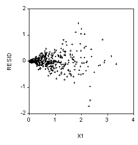
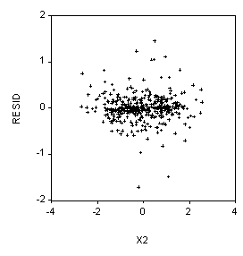
LS(H) Y C X1 X2
Or, if the correct weights are known, perform weighted least squares.
7. (5 Points) Suppose we have two variables, Y and X, and we wish to estimate the model:

What commands in EVIEWS would we use to perform the estimation?
LS (1/Y) C (1/X)
Probability and Statistics Name_________________________________
8. (10 Points) Suppose Y is the per capita consumption of ice cream in kilograms, X1 is the price of ice cream in real dollars, X2 is the per capita income in real dollars, and X3 is time measured in years (Y > 0; X1 > 0; X2 > 0). We estimate the model:
ln(yi ) = b 0 + b 1ln(Xi1 ) + b 2ln(Xi2 ) + b 3Xi3 + e i
a) (5 Points) What should the signs be (i.e., positive or negative) on b 1 and b 2 ?
b 1 < 0 and b 2 > 0
b) (5 Points) What is the interpretation -- in terms of economic theory -- of b 1, b 2, and b 3?
b 1 is the estimated price elasticity, b 2 is the estimated income elasticity, and b 3 is the growth rate of consumption with respect to time. That is, a one unit change in time (here one year) implies an approximate b 3 percent change in consumption (all else held constant).
Probability and Statistics Name_________________________________
9. (5 Points) Below is a plot of some economic data gathered over time. What EVIEWS commands (and in what order) would you use to analyze it?
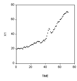
IDENT(5) D(Y) – look at the Correlogram of the first differences. OR, perhaps:
IDENT(5) DLOG(Y) – look at the Correlogram of the first differences of the natural logs.
Then, depending upon what the Correlogram shows, run models like:
LS D(Y) C MA(1), LS DLOG(Y) C MA(1), LS DLOG(Y) C AR(1) AR(2),
Etc. etc.
Probability and Statistics Name_________________________________
10. (10 Points) Consider the model of teenage drunk driving fatalities shown on page XI-6 of Epple Notes XI. Test the linear restrictions that the Protestant and Southern Baptist independent variables have the same coefficient and that the coefficient for Mormon is twice that for Catholic. Report the relevant statistic and p-value.
====================================================
Wald Test:
Equation: Untitled
====================================================
Null HypothesisC(8)=2*C(10)
               C(9)=C(11)
====================================================
F-statistic     0.364645    Probability     0.694728
Chi-square      0.729291    Probability     0.694443
====================================================
NOTE: WE ALSO ACCEPTED THE ANSWER IF YOU DID THE TWO SEPARATELY!! THAT IS,
C(8)=2*C(10) THEN THE SEPARATE TEST C(9)=C(11).
Probability and Statistics Name_________________________________
11. (10 Points) Consider the linear model below. Suppose X1 is a random variable, the correlation X2 and X3 is .9, and e is not normally distributed. How will these problems affect our estimators?
y = b 0 + b 1X1 + b 2X2 + b 3X3 + e
The estimators of b 1 and b 2 and b 3 will all be unbiased. If the mean of e is not zero, then this will be picked up by b 0 so it will be biased in that case.
Specifically, X1 random has no effect as long as X1 is not correlated with the error term.
If e is not normally distributed this also has no effect as long as there is a large number of observations (we can then appeal to the Central Limit Theorem).
X2 and X3 correlated – multicollinearity. This will affect the standard errors but the betas will still be unbiased.
Probability and Statistics Name_________________________________
12. (5 Points) Consider the correlogram below. This series was generated by an autoregressive process. What is the order of the process (that is, what is p equal to)?
AR(2), p = 2
Correlogram of Y
==============================================================
Date: 04/17/98   Time: 21:22
Sample: 1 100
Included observations: 100
==============================================================
 Autocorrelation Partial Correlation  AC     PAC  Q-Stat Prob
==============================================================
      . |*******|      . |*******|  1 0.800 0.800 65.963 0.000
      . |****** |      . |****   |  2 0.770 0.559 127.60 0.000
      . |*****  |      . | .     |  3 0.671-0.035 174.96 0.000
      . |*****  |      . | .     |  4 0.617 0.007 215.44 0.000
      . |****   |      . | .     |  5 0.571 0.061 250.40 0.000
==============================================================
13. (5 Points) Consider the correlogram below. This series was generated by a moving average process. What is the order of the process (that is, what is q equal to)?
MA(1), q = 1
Correlogram of Y
==============================================================
Date: 04/17/98   Time: 21:45
Sample: 2 100
Included observations: 99
==============================================================
 Autocorrelation Partial Correlation  AC     PAC  Q-Stat Prob
==============================================================
   *****| .     |   *****| .     |  1-0.516-0.516 27.117 0.000
      . | .     |     ***| .     |  2-0.034-0.408 27.235 0.000
      . |*.     |      **| .     |  3 0.075-0.261 27.825 0.000
      . | .     |      **| .     |  4-0.048-0.245 28.064 0.000
      . |*.     |      .*| .     |  5 0.078-0.095 28.710 0.000
==============================================================
Probability and Statistics Name_________________________________
14. (10 Points) What is the most important error you can make in a regression analysis and what can you do about it?
Specification Error. The only thing you can do about it is to improve your substantive understanding of the problem (area) you are working on.
(After specification error, the most serious problem is if the error term is correlated with the RHS variables.)