#
#
# mdscal_color_1.r -- Tests R Version of Kruskal MDS
#
#           This needs MASS and pcurve packages
#
# The Data Must Be Transformed to Squared Distances Below
#
library(MASS)
library(pcurve)
#
T <- matrix(scan("D:/R_Files/colors.txt",0),ncol=14,byrow=TRUE)
colornames <- read.csv("D:/R_Files/color_coords.txt",header=T,row.names=1)
attach(colornames)
TT <- T
nrow <- length(T[,1])
ncol <- length(T[1,])
xrow <- NULL
xcol <- NULL
matrixmean <- 0
#
# Transform the Matrix into Squared Distances The R MDS program assumes that
#                                             the data are distances
i <- 0
while (i < nrow) {
  i <- i + 1
  j <- 0
  while (j < ncol) {
     j <- j + 1
     TT[i,j] <- ((100 - T[i,j])/50)**2
  }
}
T <- TT
#
#  Kruskal MDS Routine
#
# T -- Input
# dim=2 -- number of dimensions
# maxit = number of iterations
# The program returns the configuration in points and the Stress in stress:
#     for example, colormds$points and colormds$stress
#
colorsmds <- isomds(T,dim=2, maxit=50)
#
#
plot(colorsmds$points[,1],colorsmds$points[,2],type="n",asp=1,
     main="The Color Circle\nFrom MDS Program in R",
     xlab="First Dimension",ylab="Second Dimension",
     xlim=c(-3.0,3.0),ylim=c(-3.0,3.0))
text(colorsmds$points[,1],colorsmds$points[,2],labels=row.names(colornames),adj=0)
text(-2.0,2.5,paste("Stress = ",
                0.01*round(colorsmds$stress, 2)),col="blue")
#Note this neat trick -- Stress is returned as a percentage so that
#multiplying it by 0.01 converts it to the KYST style.  The "round(..)" command
#gets us 4 digits after the decimal point
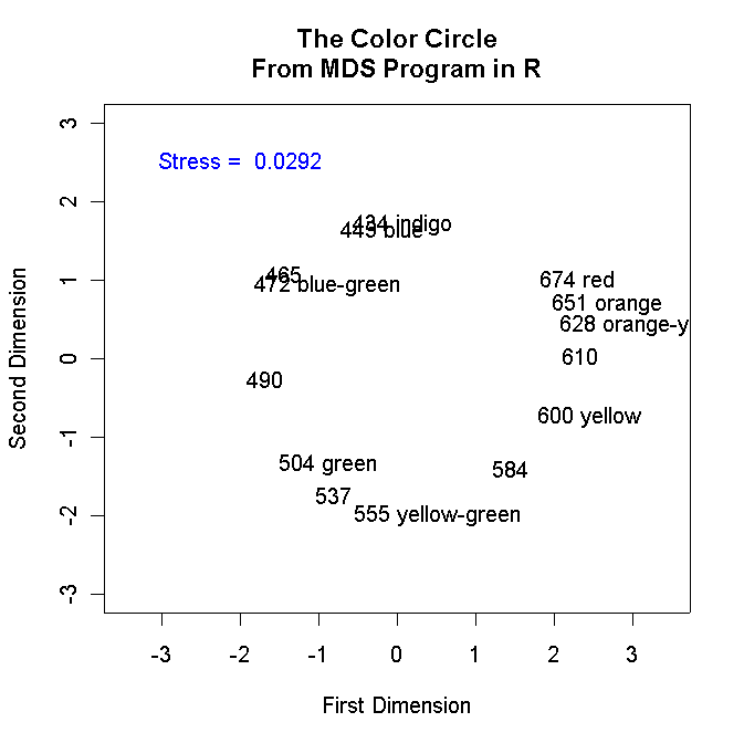
Below is the graph that the program generates:
-
Repeat problem 1a of Homework 4 using
mdscal_color_1.r. Namely, run Tables 1.1
(crime data), 1.3 (nations data), 1.4 (one spoked wheels), 4.1 (color data),
and 4.4 (Faces data -- note that these are distances!) in one,
two, and three dimensions. Produce two-dimensional plots for each
dataset and make a table showing the Stress in one, two, and three
dimensions for isomds(...) and
KYST for all the matrices. Notes:
- You have already run
KYST on all the above matrices except 4.4.
- You will have to use Epsilon
to change Tables 1.1, 1.3, 1.4, and 4.4 into square symmetric
matrices!
- To run mdscal_color_1.r in one dimension,
simply comment out the plotting commands!
- If the input data are distances/dissimilarites simply comment out the
transformation line.
Below is a listing of the program:
#
# mdscal_color_3.r -- Tests R Version of Kruskal MDS -- This version
#                      Produces Shepard's Gradient of Generalization
#
#           This needs MASS and pcurve packages
#
# The Data Must Be Transformed to Squared Distances Below
#
library(MASS)                   Note that this program is the same as the one
library(pcurve)                 above through the call to isomds(...)
#
T <- matrix(scan("F:/R_Files_Office/colors.txt",0),ncol=14,byrow=TRUE)
colornames <- read.csv("F:/R_Files_Office/color_coords.txt",header=T,row.names=1)
attach(colornames)
TT <- T
#
#  Save Copy of Original Data
#
TTT <-T
nrow <- length(T[,1])
ncol <- length(T[1,])
#
y <- rep(0,((nrow*(nrow+1))/2)*5)   This simply creates a matrix that will hold
dim(y) <- c(((nrow*(nrow+1))/2),5)  the "DATA" and "DIST" as in KYST
#
#
# Transform the Matrix to Squared Distances
#
i <- 0
while (i < nrow) {
  i <- i + 1
  j <- 0
  while (j < ncol) {
     j <- j + 1
#
#  Adjust This Transformation According to the MAXIMUM similarity
#    Value!  The Diagonal of the Matrix Should be all zeroes!
#    If the data are correlations this would be:
#     TT[i,j] <- (1.0 - T[i,j])**2
#    If the maximum value for the Similarity was 10 this would be:
#     TT[i,j] <- (10.0 - T[i,j])**2 or
#     TT[i,j] <- ((10.0 - T[i,j])/5.0)**2
#
     TT[i,j] <- ((100 - T[i,j])/50)**2
  }
}
T <- TT
#
#
# T -- Input
# dim=2 -- number of dimensions
#
dim <- 2
colorsmds <- isomds(T,dim, maxit=50)
#
#
# Create Data for Gradient of Generalization Plots
#
i <- 1                           This code creates the Euclidean distances
kk <- 0                          between the points estimated by isomds(...).
while (i <= nrow) {              These are stored in the matrix y(,) along with
  j <- i                         the original Similarities and the Dissimilarities
  while (j <= nrow) {            computed above.
     k <- 0
     dist <- 0.0
     while (k < dim) {
       k <- k+1
       dist <- dist + (colorsmds$points[i,k]-colorsmds$points[j,k])^2
     }
     kk <- kk +1
     y[kk,1] <- dist
     y[kk,2] <- T[i,j]
     y[kk,3] <- TTT[i,j]
     y[kk,4] <- i
     y[kk,5] <- j
  j <- j + 1
  }
  i <- i + 1
}
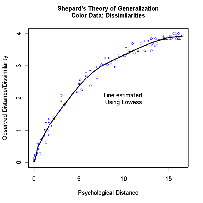
#             This produces a plot of the Distances against the Dissimilarities
plot(y[,1],y[,2],
     xlab="Psychological Distance",ylab="Observed Distance/Dissimilarity",col="blue")
mtext(side=3,line=1.5,"Shepard's Theory of Generalization\nColor Data: Dissimilarities",font=2)
lines(lowess(y[,1],y[,2],f=.2),lwd=3)
text(10,2,"Line estimated \nUsing Lowess")
#
windows()               This Command allows us to create the second plot
#                       The Last One Drawn will be on Top
#
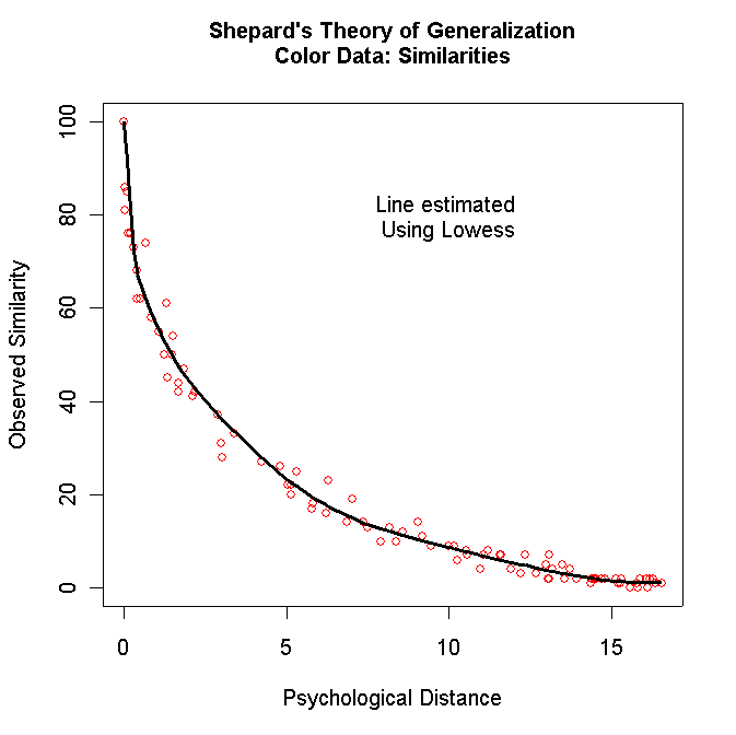
#             This produces a plot of the Distances against the Similarities
plot(y[,1],y[,3],ylim=c(0,100),
     xlab="Psychological Distance",ylab="Observed Similarity",col="red")
mtext(side=3,line=1.5,"Shepard's Theory of Generalization\nColor Data: Similarities",font=2)
lines(lowess(y[,1],y[,3],f=.2),lwd=3)
text(10,80,"Line estimated \nUsing Lowess")
For the color data, you should get the following two graphs:

Turn in both graphs for each matrix except for the Faces data (Table 4.4). Just turn in the Dissimilarities against the Distances plot for the Faces data (you can comment out the code for the other plot for this data).
VOTE_THERM_2000.ORD
NON-PARAMETRIC MULTIDIMENSIONAL UNFOLDING OF THERMOMETER DATA
    1   91   20   40    2
(40A1,3900I1)
(I5,1X,40A1,2I5,50F8.3)
We are going to use a modified version of
Optimal Classification more suited to analyzing
roll calls from rank order data. The program is PERFLRANK.
Download the program and place it in the same directory as your PERFSTRT.DAT and
the candidate "roll call" file VOTE_THERM_2000.ORD.-
Run PERFLRANK using the above PERFSTRT.DAT and
VOTE_THERM_2000.ORD. Turn in the PERF21.DAT file.
The PERF25.DAT shows the rank ordering of the 1,443 respondents included in the scaling along with the rank positions of the cutpoints for the candidate "roll calls." Note that because tied ranks are allowed, the respondents are ordered from 17.5 to 1,419.5. The respondents are first shown in their rank ordering from 17.5 to 1,419.5 and then in the order that they appear in VOTE_THERM_2000.ORD. The 91 cutpoints corresponding to the candidate "roll calls" are at the bottom of PERF25.DAT and the rank position of the cutpoints are in the last column. This part of the file looks like this:
    1    1 436 568 291  0.333 1 6   392.500
    2    2 691 609  80  0.869 1 6   809.000
    3    3 781 369  99  0.732 1 6  1114.000
    4    4 515 453 191  0.578 1 6  1058.750
    5    5 503 539 166  0.670 1 6   688.000
    6    6 494 462 178  0.615 1 6   922.500
    7    7 428 463 212  0.505 1 6   797.750
    8    8 558 488  84  0.828 1 6   809.000
    9    9 588 427 328  0.232 6 1   171.000
   10   10 422 604 340  0.194 1 6   779.250
   11   11 720 567  65  0.885 1 6   788.250
   12   12 662 313  95  0.696 1 6  1047.250
   13   13 693 504 151  0.700 1 6   797.750
             etc etc etc
   85   85 633 573 169  0.705 1 6   715.750
   86   86 678 488  60  0.877 1 6   896.750
   87   87 707 235  91  0.613 1 6  1199.000
   88   88 701 387 110  0.716 1 6   980.750
   89   89 644 265 117  0.558 6 1   359.000
   90   90 565 468 147  0.686 6 1   602.000
   91   91 249 600 208  0.165 6 1  1349.500
Use Epsilon to merge in the 91
pairs of candidate names that you created in
question 1.a of Homework number 10 into this file.
The first 13 lines of your file should look exactly like this!!!
 CLINTON      GORE              1 436 568 291  0.333 1 6   392.500
 CLINTON      BUSH              2 691 609  80  0.869 1 6   809.000
 CLINTON      BUCHANAN          3 781 369  99  0.732 1 6  1114.000
 CLINTON      NADER             4 515 453 191  0.578 1 6  1058.750
 CLINTON      MCCAIN            5 503 539 166  0.670 1 6   688.000
 CLINTON      BRADLEY           6 494 462 178  0.615 1 6   922.500
 CLINTON      LIEBERMAN         7 428 463 212  0.505 1 6   797.750
 CLINTON      CHENEY            8 558 488  84  0.828 1 6   809.000
 CLINTON      HILLARY           9 588 427 328  0.232 6 1   171.000
 CLINTON      DEMPARTY         10 422 604 340  0.194 1 6   779.250
 CLINTON      REPUBPARTY       11 720 567  65  0.885 1 6   788.250
 CLINTON      REFORMPTY        12 662 313  95  0.696 1 6  1047.250
 CLINTON      PARTIES          13 693 504 151  0.700 1 6   797.750
                       etc etc etc
Turn in the Epsilon macro you used to create your
file and a complete listing of the file.There are 13 cutpoints associated with former President Clinton. The cutpoint between former President Clinton and former Vice-President Gore is 392.5. The "1 6" to the immediate left of the rank tells you that Yea (vote for Clinton) was below 392.5 and Nay (vote for Gore) was above 392.5. This implies that former President Clinton's rank position is below 392.5 and former Vice-President Gore's rank position is above 392.5. Although the data has some noise in it, you should be able to pin down a range within which former President Clinton's rank should lie. For example, note that the cutpoint between former President Clinton and Hillary Clinton is 171.0 and the "6 1" means that Hillary Clinton is below 171.0 and former President Clinton is is above 171.0.
Using the above reasoning, locate a range of ranks for former President Clinton, former Vice-President Gore, President Bush, and Hillary Clinton. Defend you reasoning for each person!
Use Epsilon to merge the "vote for" variable in VOTE_THERM_2000.ORD into the respondent rank file (cut the respondents out of PERF25.DAT first). Turn in a listing of the Epsilon macro you use to create the file.
Make smoothed histograms of the Bush and Gore voters from the above file. These histograms should look similar to those you made in question 1.c of Homework 8.