Below is a listing of the program and the graph that it creates:
#
#  Program to Illustrate Singular Value Decomposition
#
#      Draws n points from bivariate normal distribution
#         and draws graph of ratio of 1st over 2nd
#         Singular Values
#
nrow <- 1000
ncol <- 2
#
#  Number of Iterations
#
nitr <- 39
#
#  These two commands create a matrix that is 39 by 4 and filled
#   with zeroes
#
w <- rep(0,nitr*4)
dim(w) <- c(nitr,4)
#
#  xinc is the increment -- that is, the value that is subtracted
#    from the previous value of the correlation after every pass
#    through the loop below.  Note that it equals .05
#
xinc <- 2/(nitr+1)
#
#  Initial Value for Correlation
#
rcor <- .95
#
#  Note that at the first pass through the loop r=.95, the 2nd pass
#    r=.90, third pass r=.85, etc.  At the 39th pass, r=-.95.
#
iii <- 1
while (iii <= nitr) {
#
#  Create Variance-Covariance Matrix
#
#         1.0  0.9
#         0.9  1.0
#
Sigma <- matrix(c(1,rcor,rcor,1),2,2)
#
#  Call Bivariate Normal with zero mean and
#   Sigma Var-Cov Matrix, Place in X
#
X <- mvrnorm(n=nrow,rep(0,2),Sigma)
#
#  Perform Singular Value Decomposition
#
xsvd <- svd(X)
#
#  The Two Lines Below Put the Singular Values in a
#    Diagonal Matrix -- The first one creates an
#    identity matrix and the second command puts
#    the singular values on the diagonal
#
Lambda <- diag(ncol)
diag(Lambda) <- xsvd$d
#
#  Compute U*LAMBDA*V' for check below
#
XX <- xsvd$u %*% Lambda %*% t(xsvd$v)
#
# Compute Fit of SVD -- This is just the sum of squared
#  error -- Note that ssesvd should be zero!
#
#
i <- 0
j <- 0
ssesvd <- 0
while (i < nrow) {
  i <- i + 1
  j <- 0
  while (j < ncol) {
     j <- j + 1
     ssesvd <- ssesvd + (X[i,j] - XX[i,j])**2
  }
}
#
#  Store the correlation, fit, and two singular values for plotting
#   purposes
#
w[iii,1] <- rcor
w[iii,2] <- ssesvd
w[iii,3] <- xsvd$d[1]
w[iii,4] <- xsvd$d[2]
#
#  Increment correlation value
#
rcor <- rcor - xinc
#
#  Increment Loop counter
#
iii <- iii+1
#
# End of Big Loop
#
}
#
#  Plot Commands
#
plot(w[,1],w[,3]/w[,4],xlab="Correlation Between Dimensions",ylab="Ratio of 1st to 2nd Singular Value",pch=16,col="blue")
mtext(side=3,line=1.5,"Bivariate Normal Random Draws \nRatio of Singular Values",font=2)
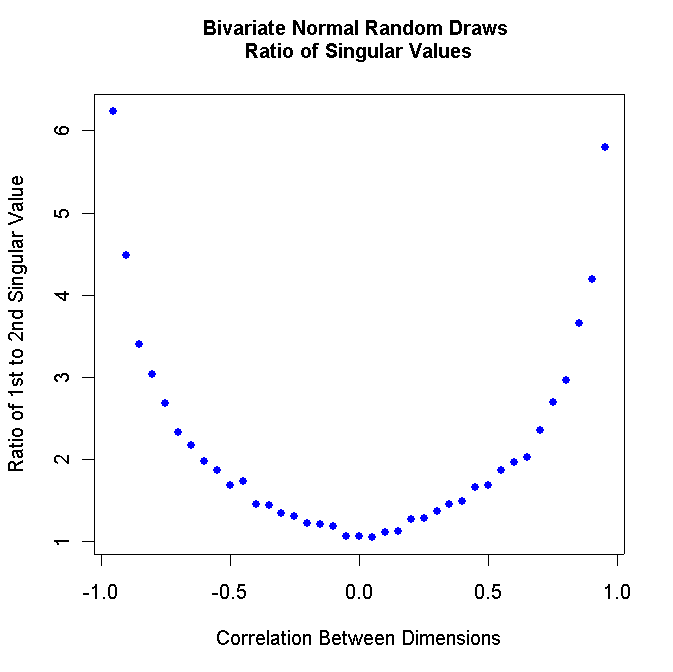
Note that the figure above is symmetric! Consequently, we only need to be concerned with studying correlation values between zero and 1.0.
-
Modify the R program above so that it
runs from .98 to .00 in steps of .02. Turn in your program listing and turn in
the resulting graph. It should look something like this:
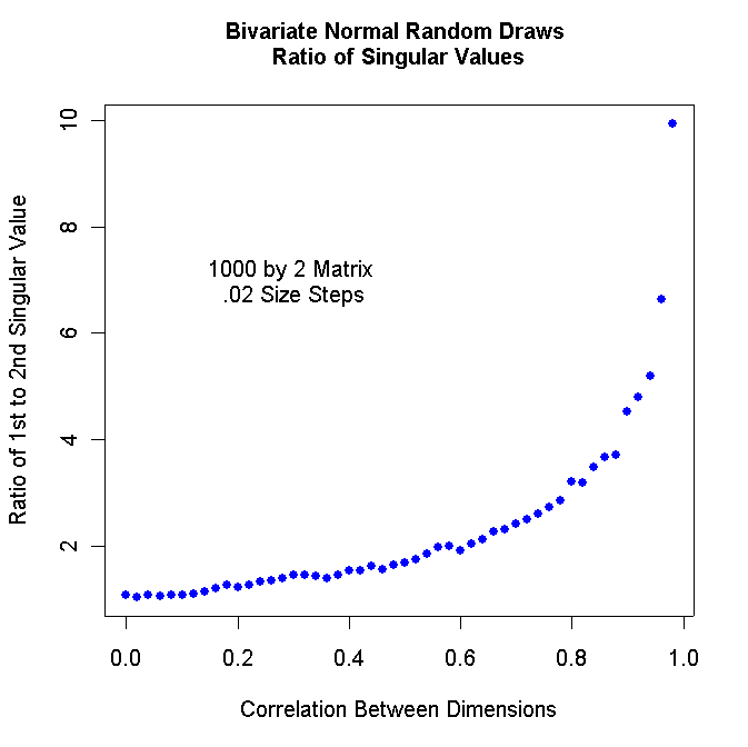
You can insert text inside the graph with the command:
text(.3,7.0,"1000 by 2 Matrix \n.02 Size Steps")
Run your R program from .99 to .00 in steps of .01. Turn in the graph.
Run your R program from .98 to .00 in steps of .02 with 2000 by 2 matrices. Turn in the graph.
Run your R program from .98 to .00 in steps of .02 with 5000 by 2 matrices. Turn in the graph.
Run your R program from .99 to .00 in steps of .01 with 100 by 2 matrices. Turn in the graph.
The first few lines of the agreement score file SEN107.DAT should look like this:
1079991099 0USA     200  BUSH        100  92  92  99  97  96  etc etc
1074970041 0ALABAMA 20001SESSIONS     92 100  92  89  86  86  etc etc
1079465941 0ALABAMA 20001SHELBY       92  92 100  90  87  83  etc etc
                      etc etc etc
Use Epsilon to strip off the header of each
row so that you only have the agreement score matrix itself. Download the
double-centering program below:Below is a listing of the program:
#
# double_center_6.r -- Double-Center Program
#
# The Data Are assumed to be Squared Distances -- Data Must
#     Be Transformed to Squared Distances Below
#
T <- matrix(scan("D:/R_Files/sen107_ascore.dat",0),ncol=103,byrow=TRUE)
sennames <- read.csv("D:/R_Files/sen_107.txt",header=F)
attach(sennames)
#
#  Catch The Missing Data
#
TT <- ifelse(T <= 0,50,T)
T <- TT
#
#
nrow <- length(T[,1])
ncol <- length(T[1,])
xrow <- NULL
xcol <- NULL
matrixmean <- 0
matrixmean2 <- 0
#
# Transform the Matrix
#
i <- 0
while (i < nrow) {
  i <- i + 1
  j <- 0
  while (j < ncol) {
     j <- j + 1
#
#  This is the Normal Transformation
#
     TT[i,j] <- ((100 - T[i,j])/50)**2
#
  }
}
T <- TT
#
#
# Compute Row and Column Means
#
i <- 0
while (i < nrow) {
  i <- i + 1
  xrow[i] <- mean(T[i,])
}
i <- 0
while (i < ncol) {
  i <- i + 1
  xcol[i] <- mean(T[,i])
}
matrixmean <- mean(xcol)
matrixmean2 <- mean(xrow)
#
# Double-Center the Matrix
#
i <- 0
while (i < nrow) {
  i <- i + 1
  j <- 0
  while (j < ncol) {
     j <- j + 1
     TT[i,j] <- (T[i,j]-xrow[i]-xcol[j]+matrixmean)/(-2)
  }
}
ev <- eigen(TT)
DIM.1 <- ev$vec[,1]*sqrt(ev$val[1])
DIM.2 <- ev$vec[,2]*sqrt(ev$val[2])
#
SEN107_ASCORE.DAT is the agreement score matrix and
SEN_107.TXT has the roll call vote. For example, here is the first
few lines of my SEN_107.TXT file:
 99,USA    , 200,1,Bush
 41,ALABAMA, 200,1,Sessions
 41,ALABAMA, 200,1,Shelby
 81,ALASKA , 200,1,Murkowski
 81,ALASKA , 200,1,Stevens
 61,ARIZONA, 200,1,Kyl
 61,ARIZONA, 200,1,McCain
 42,ARKANSA, 200,0,Hutchinson
 42,ARKANSA, 100,6,Lincoln
 71,CALIFOR, 100,6,Boxer
    etc etc etc
Note that I use "1" for Yea, "6" for Nay, and "0" for no longer
in the Senate. I also treated President Bush as if he voted for
Cloture.-
Construct the SEN_107.TXT file and turn in a listing
of it.
Produce a Density plot of the Yea and Nay voters on the Cloture vote for the Estrada nomination. If you do it correctly, it should look something like the following:
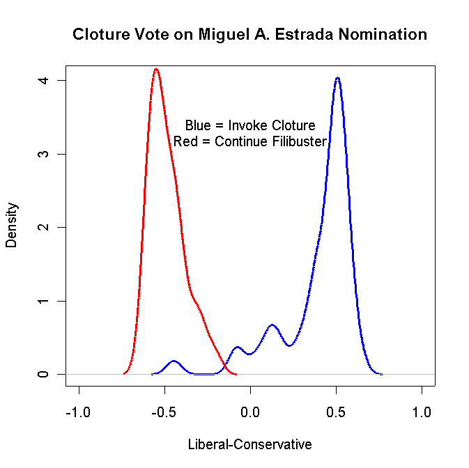
Turn in your graph and the R code that you used to create the graph.
Produce a Density plot of the Democrat Yea and Nay voters on the Cloture vote for the Estrada nomination. If you do it correctly, it should look something like the following:
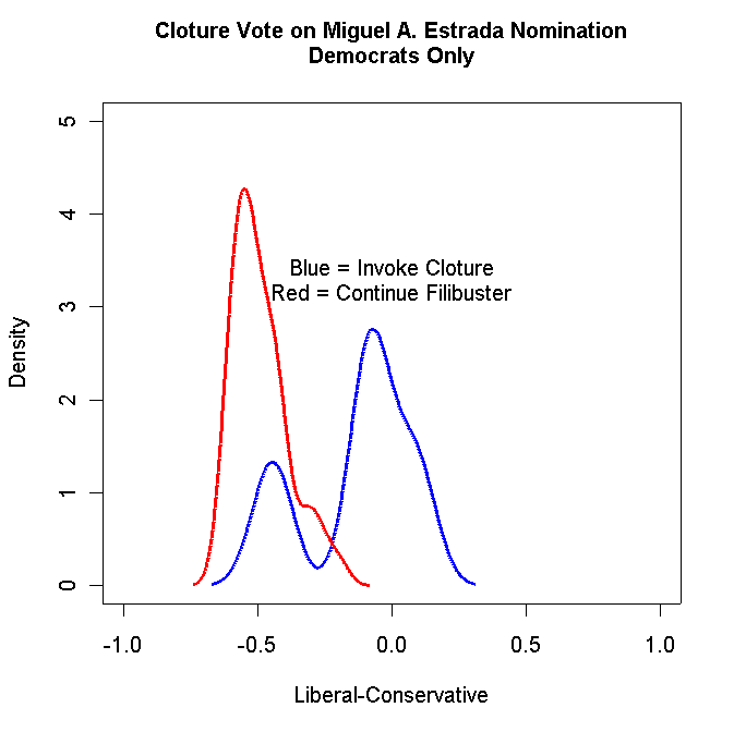
Turn in your graph and the R code that you used to create the graph.
The 1968 Election Data file contains the same variables that we have used in the past plus the thermometer scores and voting information for the respondents. The variables are:
idno           respondent id number
partyid        strength of party id -- 0 to 6
income         raw income category
incomeq        income quintile -- 1 to 5
race           0 = white, 1 = black
sex            0 = man, 1 = woman
south          0 = north, 1 = south
education      1=HS, 2=SC, 3=College
age            age in years
uulbj          lbj position urban unrest
uuhhh          humphrey pos urban unrest
uunixon        nixon position urban unrest
uuwallace      wallace pos urban unrest
uuself         self placement urban unrest
vnmlbj         lbj pos vietnam
vnmhhh         hhh pos vietnam
vnmnixon       nixon pos vietnam
vnmwallace     wallace pos vietnam
vnmself        self placement vietnam
voted          1=voted, 5=did not vote
votedfor       who voted for -- 1 = humphrey, 2= nixon, 3=wallace
wallace        wallace therm
humphrey       humphrey thermometer
nixon          nixon thermometer
mccarthy       mccarthy thermometer
reagan         reagan thermometer
rockefeller    rockefeller thermometer
lbj            lbj thermometer
romney         romney thermometer
kennedy        robert kennedy thermometer
muskie         muskie thermometer
agnew          agnew thermometer
lemay          "bombs away with Curtis LeMay" thermometer
The control card file for the metric unfolding procedure is shown below. The first line has the name of the data file. The first number in the second line is the number of stimuli, the next two numbers are the minimum and maximum number of dimensions to estimate, and the "10" is the number of iterations.
The third line contains some "antique" options we will never use. The only numbers that matter on this line are the "4" which indicates the number of identifying characters to read off each line of the data file (e.g., the respondent id number), and the "2" at the end. This is the number of missing data codes which appear in the sixth line.
The first number in the fourth line is a tolerance value -- leave it as is. The next three numbers are parameters to transform the input data into squared distances. In this case, let amx=-.02, bmx=2.0, and cmx=2.0. The following equation transforms the thermometers into squared distances:
d2 = (amx*t+bmx)cmx
where t = input data. This formula takes a linear transformation of the input data to the power cmx. With amx = -.02, bmx = 2.0, and cmx = 2.0, this is equivalent to subtracting the thermometer score from 100, dividing by 50, and then squaring. This converts t from a 0-100 scale to a 4-0 scale. If the data, t, are distances, set amx = 1.0, bmx = 0.0, and cmx = 2.0. If the data are correlations, set amx = -1.0, bmx = 1.0, and cmx=2.0 or 1.0 if the correlations are initially regarded as unsquared or squared distances respectively.
The next value, "1.5", is the maximum absolute expected coordinate value on any dimension. It is used for plotting purposes. If the squared distances are confined to a 4-0 scale, xmax=1.5 is usually sufficient. The last two numbers, "0.0" and "100.0", are the minimum and maximum expected values of the input data. These are used to catch coding errors in the input data. Anything out of range is treated as missing data.
The fifth line is the format of the data file and the sixth line contains the missing data codes.
Finally, the last 12 lines are labels for the stimuli.
OLS68B.DAT
   12    2    2   10    0    0
    1    1    0    4    2
    .001  -0.02    2.0     2.0     1.5     0.0   100.0
(1X,4A1,60X,12F3.0)
 98 99
WALLACE
HUMPHREY
NIXON
MCCARTHY
REAGAN
ROCKEFELLER
LBJ
ROMNEY
R.KENNEDY
MUSKIE
AGNEW
LEMAY
-
Run MLSMU6. It will produce an output
file called FORT.22. The first 20 lines look like this:
 WALLACE          1.2646    0.5154  217.4823    0.5541 1242.0000
 HUMPHREY        -0.5559    0.3738  114.7892    0.6968 1252.0000
 NIXON            0.1480   -0.5415  123.2209    0.5319 1250.0000
 MCCARTHY        -0.6251   -0.4938  151.8926    0.3854 1204.0000
 REAGAN           0.3080   -0.8895  131.8091    0.4380 1212.0000
 ROCKEFELLER     -0.5579   -0.5995  148.1413    0.3724 1229.0000
 LBJ             -0.5223    0.4905  147.0334    0.5573 1253.0000
 ROMNEY          -0.4736   -0.7866  111.3147    0.3434 1167.0000
 R.KENNEDY       -0.4245    0.2351  148.8571    0.5418 1242.0000
 MUSKIE          -0.6611    0.1660  126.0836    0.4862 1177.0000
 AGNEW            0.2341   -0.8706  114.1418    0.4675 1180.0000
 LEMAY            1.1901    0.4267  174.3242    0.4601 1188.0000
 1681            -0.0285    0.2555    0.7918    0.6824   12.0000
 1124            -0.1768    0.2692    1.4788    0.6992   12.0000
   78             0.5707   -0.1514    3.5611    0.2141   12.0000
  553             0.1376    0.1064    0.1597    0.7047    9.0000
    7             0.2542    0.1235    1.2634    0.0116   12.0000
  412             0.2781    0.0867    0.1024    0.6197   12.0000
  631             0.5017    0.1088    1.1196    0.0742   12.0000
 1316             0.2175   -0.5842    1.1568    0.8577   12.0000
                       etc etc etc
                       etc etc etc
The first two columns after the names are the two dimensional coordinates. The first
12 lines are the coordinates for the political candidates and lines 13 onward are the
coordinates for the respondents. Use R to plot the
12 candidates in two dimensions. This plot should be very similar to the one
you did for question 2 of homework 5.Use Epsilon to insert the voted and voted for variables into FORT.22 (strip off the candidate coordinates first). Turn in the Epsilon macro you used to do the insertion and the first 20 lines of the file.
Use R to make two-dimensional plots of the Voters, Non-Voters, Humphrey Voters only, Nixon Voters only, and Wallace Voters only. For example, your Humphrey Voter plot should look something like this:
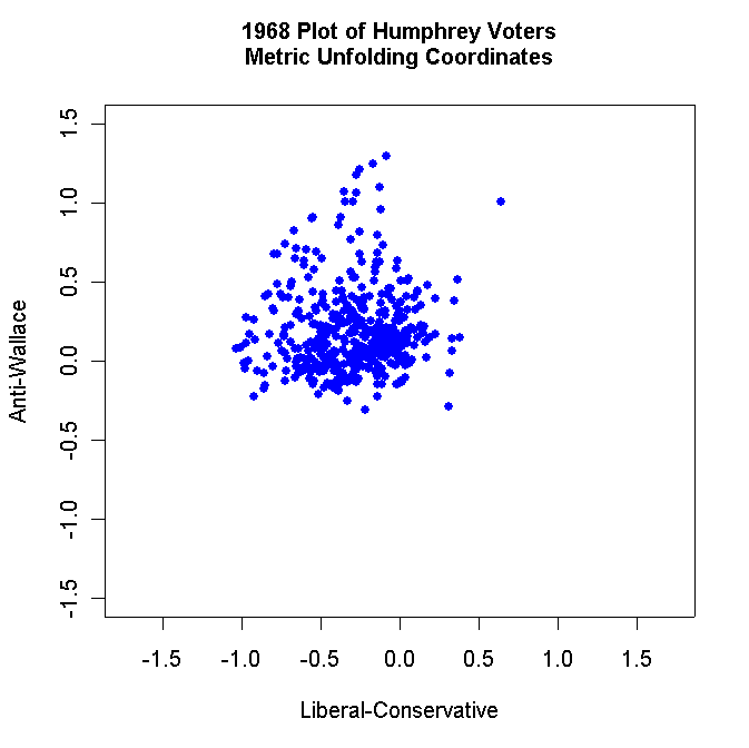
Label each plot appropriately and use solid dots to plot the respondents. Turn in all these plots.