POLS 6386 MEASUREMENT THEORY
Eighth Assignment
Due 25 March 2003

1. The aim of this homework is to compare the polarization in the mass public with that in Congress. In this part of the homework we will use the Aldrich-McKelvey scaling program to analyze the Liberal-Conservative 7-Point Scale from the 2000 election study. Download the program and the 2000 data and "control card" files:
   
   Aldrich-McKelvey scaling program (Updated From Homework 6!)
   
   2000 NES Data
   
   2000 Liberal-Conservative Control Card File
   
   and place them in the same folder on a WINTEL machine. Read the Aldrich-McKelvey scaling program page to see how to run the program.
   
   Here are the first four lines of ELEC2000.DAT.

   
       10787  4  8  0  0  0  2 49  1   0  65  60  30  40  70  50 998 998  40  59  75  63  65  6  1  3  6  4  0  2
       21271  2  6  0  1  0  2 35  1  50  50  50  50 997  50   0  50 997  50 100   0 100   0  4  4  2  6  8  0  0
       40285  2  6  0  0  0  2 63  0  70  55  55  60  65  55  55  65  50  60  70  65  65  90  6  5  5  5  5  0  1
       50191  6  6  0  1  0  2 40  1  50  40  80  60  60  80  70  50  70   0  20  90  70  70  6  2  2  6  4  0  2
   
   The variables, in order, are:
   
       RESPONDENT ID      = unique 8 digit number
       PARTY ID           = 0 to 6 -- 0 = Strong Democrat
                                      1 = Weak Democrat
                                      2 = Lean Democrat
                                      3 = Independent
                                      4 = Lean Republican
                                      5 = Weak Republican
                                      6 = Strong Republican
       FAMILY INCOME      = 1 to 22 - 1.   A. NONE OR LESS THAN $4,999
                                      2.   B. $5,000-$9,999
                                      3.   C. $10,000-$14,999
                                      4.   D. $15,000-$24,999
                                      5.   E. $25,000-$34,999
                                      6.   F. $35,000-$49,999
                                      7.   G. $50,000-$64,999
                                      8.   H. $65,000-$74,999
                                      9.   J. $75,000-$84,999
                                      10.  K. $85,000-$94,999
                                      11.  M. $95,000-$104,999
                                      12.  N. $105,000-$114,999
                                      13.  P. $115,000-$124,999
                                      14.  Q. $125,000-$134,999
                                      15.  R. $135,000-$144,999
                                      16.  S. $145,000-$154,999
                                      17.  T. $155,000-$164,999
                                      18.  U. $165,000-$174,999
                                      19.  V. $175,000-$184,999
                                      20.  W. $185,000-$194,999
                                      21.  X. $195,000-$199,999
                                      22.  Y. $200,000 and over
                               
       RACE               = 0 White, 1 Black
       SEX                = 0 Man, 1 Woman
       SOUTH              = 0 North, 1 South
       EDUCATION          = 1 High School or less, 2 Some College, 3 College
       AGE                = In Years
       MARRIED            = 0 Single, 1 Married
   
       FEELING THERMOMETERS   (0 TO 100)
   
                          = CLINTON  
                          = GORE     
                          = BUSH     
                          = BUCHANAN 
                          = NADER    
                          = MCCAIN   
                          = BRADLEY  
                          = LIEBERMAN
                          = CHENEY   
                          = HILLARY CLINTON
                          = DEMOCRATIC PARTY
                          = REPUBLICAN PARTY
                          = REFORM PARTY
                          = PARTIES IN GENERAL
       
       LIBERAL-CONSERVATIVE  SCALE  (1=EXTREMELY LIBERAL, 2=LIBERAL, 3=SLIGHTLY LIBERAL,
                                4=MODERATE; MIDDLE OF THE ROAD, 5=SLIGHTLY CONSERVATIVE,
                                6=CONSERVATIVE, 7=EXTREMELY CONSERVATIVE)
   
   
                          = SELF-PLACEMENT
                          = CLINTON
                          = GORE
                          = BUSH
                          = BUCHANAN
   
       PRE-POST INTERVIEW = 1 IF PRE-ELECTION INTERVIEW ONLY
       VOTE CHOICE        = 0 NON-VOTER
                          = 1 GORE
                          = 2 BUSH
                          = 3 3RD PARTY
   

   Run the Aldrich-McKelvey scaling procedure on the 2000 election Liberal-Conservative 7-Point scale. Save the coordinate output files.
   
   
   1. Use Epsilon to merge the PARTY ID, FAMILY INCOME, RACE, SEX, and VOTE CHOICE variables from ELEC2000.DAT into the coordinate output file. For example, here are the first few lines of the coordinate output file:

      
            LINE #   CASE #  R POS   ALPHA    BETA    SCALED POS    RSQ
               1     10787   6.0   -1.0037    0.2868    0.7169    0.6136    0.7834
               4     50191   6.0   -1.1883    0.3395    0.8488    0.7278    0.8531
               5     70894   5.0   -1.0960    0.2923    0.3653    0.8212    0.9062
               6     80889   4.0   -1.5136    0.3187   -0.2390    0.8597    0.9272
               7     90892   3.0   -1.4170    0.3149   -0.4723    0.9675    0.9836

      and here are the first few lines of the coordinate output file after the variables are merged in (using a macro that I wrote):

      
               1  4  8  0  0  2    10787   6.0   -1.0037    0.2868    0.7169    0.6136    0.7834
               4  6  6  0  1  2    50191   6.0   -1.1883    0.3395    0.8488    0.7278    0.8531
               5  5 12  0  0  0    70894   5.0   -1.0960    0.2923    0.3653    0.8212    0.9062
               6  0  7  0  1  1    80889   4.0   -1.5136    0.3187   -0.2390    0.8597    0.9272
               7  0 11  0  1  1    90892   3.0   -1.4170    0.3149   -0.4723    0.9675    0.9836

      Turn in the Epsilon macro you write that inserts the above variables into the coordinate file. In the macro, use a split screen and place the coordinate file in the top screen and ELEC2000.DAT in the bottom screen.
      
      
   2. Simplify the coordinate file by deleting all the columns except for those you inserted, BETA (you will need that for graphing), and the Scaled Position. If you have done everything correctly the first few lines of your file should look like this:

      
        4  8  0  0  2     0.2868    0.7169
        6  6  0  1  2     0.3395    0.8488
        5 12  0  0  0     0.2923    0.3653
        0  7  0  1  1     0.3187   -0.2390
        0 11  0  1  1     0.3149   -0.4723
        0  6  0  1  1     0.3681   -1.0123
        5  7  0  1  1     0.1850    0.0000
                etc.
                etc.
                etc.

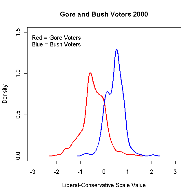
      Read the above file into R and make smoothed histograms of the scaled positions of the respondents by party ID. Replicate the graphs you did for question 2.c of homework 6. Use positive BETA respondents only in this graph and all the graphs below.
      
      
   3. Make smoothed histograms of the scaled positions of the respondents by their presidential vote (Bush and Gore). Turn in the graph and the R code you used to make your graph. It should look something like this:
      
      
      
      
   4. Make smoothed histograms of the scaled positions by Race. Turn in the graph and the R code you used to make your graph.
      
      
   5. Make smoothed histograms of the scaled positions by Sex. Turn in the graph and the R code you used to make your graph.
      
      
   6. Make smoothed histograms of the scaled positions by Low and High Income. Pick a reasonable breakpoint -- for example, $35,000 and down versus $35,000 and up. Turn in the graph and the R code you used to make your graph. Also, write a short paragraph justifying your breakpoint!!!
      
      
      
      
2. The aim of this problem is to analyze the 2000 thermometer scores using metric unfolding in the same fashion as question 3 of homework 7. Download the the program, control card file, and data file and place them in the same directory.
   
   Metric Unfolding Program (MLSMU6)
   
   Control Card File for Metric Unfolding Program
   
   2000 Election Data (Same as Problem 1 above)
   
   
   1. Run MLSMU6. It will produce an output file called FORT.22. The first 20 lines look like this:

      
       CLINTON         -0.7879   -0.0317  153.1404    0.7198 1477.0000
       GORE            -0.7133   -0.1701  112.1776    0.7061 1468.0000
       BUSH             0.8234   -0.2492  149.4325    0.5889 1458.0000
       BUCHANAN         0.4576    1.0536  178.0645    0.3114 1246.0000
       NADER           -0.2737    0.7599  174.6307    0.2645 1094.0000
       MCCAIN           0.2850   -0.6498  122.5794    0.3691 1182.0000
       BRADLEY         -0.0780   -0.7509  106.1498    0.3689 1088.0000
       LIEBERMAN       -0.3428   -0.6394  107.1314    0.4758 1096.0000
       CHENEY           0.7002   -0.4687  107.9753    0.5099 1147.0000
       HILLARY         -0.8617    0.0625  203.7540    0.6459 1466.0000
       DEMPARTY        -0.6788   -0.1713  112.8208    0.6861 1453.0000
       REPUBPARTY       0.8235   -0.3286  142.8395    0.5546 1447.0000
       REFORMPTY        0.1644    1.0398  132.9094    0.3140 1128.0000
       PARTIES          0.1949   -0.7946  158.0865    0.2290 1413.0000
          1             0.3666   -0.0534    1.2943    0.3584   12.0000
          2            -0.2740    0.6767    2.5447    0.5465   12.0000
          4             0.0094    0.0645    0.8008    0.0000   14.0000
          5             0.5073   -0.0010    1.3888    0.6249   14.0000
          7             0.2719    0.0294    0.3600    0.5458   14.0000
          8            -0.6582   -0.2931    1.8168    0.7683   14.0000
                                   etc etc etc
                                   etc etc etc

      Use R to plot the 14 stimuli in two dimensions. This plot should be very similar to the one you did for question 2 of homework 5 and question 3 of homework 7.
      
      
   2. Use Epsilon to insert the VOTE CHOICE variable into FORT.22 (strip off the candidate coordinates first). Turn in the Epsilon macro you used to do the insertion and the first 20 lines of the file.
      
      
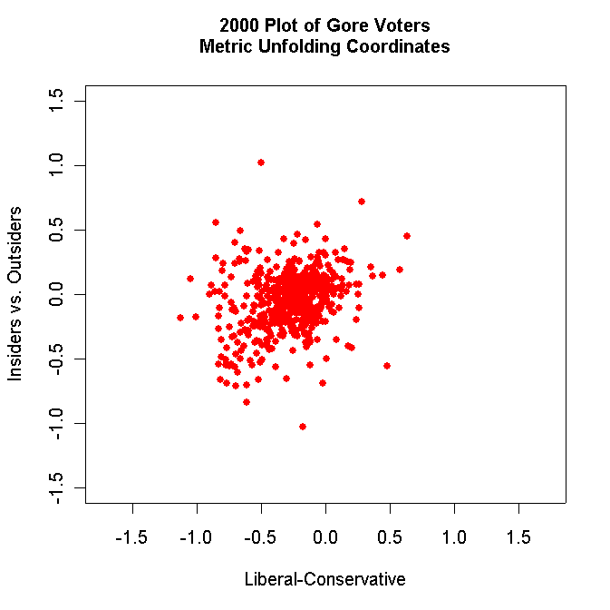
   3. Use R to make two-dimensional plots of the Voters, Non-Voters, Gore Voters only, and Bush Voters only. For example, your Gore Voter plot should look something like this:
      
      
      
      Label each plot appropriately and use solid dots to plot the respondents. Turn in all these plots.
      
      
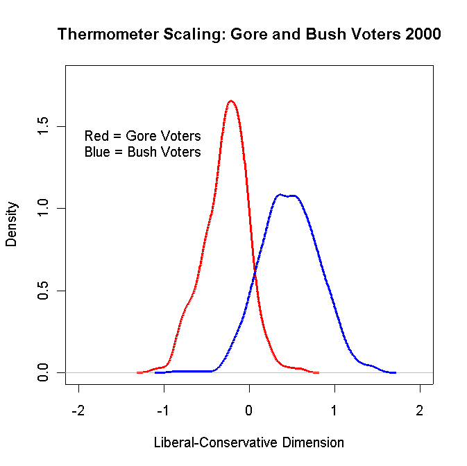
   4. Use R to make smoothed histograms -- using the first dimension from the thermometer scaling -- of the Voters and Non-Voters only, and the Gore and Bush Voters only. For example, your Gore and Bush Voter plot should look something like this:
      
      
      
      Turn in the R code and the plots.
      
      
3. The aim of this problem is to show you how to use the quadratic-normal (QN) scaling program to analyze congressional roll call data. Download the program, control card file, and the 106^th roll call data and place them in the same directory.
   
   Quadratic-Normal Scaling Program (QUADMD00)
   
   Control Card File for QN Program
   
   106^th House Roll Call Data
   
   The Control Card file -- QUADSTRT.DAT -- looks like this:

   
   HOU106KH.ORD
   QUADRATIC-NORMAL MULTIDIMENSIONAL UNFOLDING
       1 1209   10   36    1
   (36A1,3600I1)
   (I5,1X,36A1,2I5,50F8.3)
   (I5,1X,36A1,2I5,F8.3,F12.3,50F8.3)

   The first line has the name of the data file. The second line, in order, is the number of dimensions to estimate, the number of roll calls, the number of iterations for the program to run, the number of characters on the header of each line of the input file, and the last number tells the program to put that legislator on the left (i.e., less than zero -- in this instance, former President Clinton).
   
   The legislator coordinates are in the output file QUAD0048.DAT. The first ten lines look like this:

   
       1 1069990999 0USA     100  CLINTON       80   15   0.842     -33.626   0.702  -0.993   2.381   0.184
       2 1061509041 1ALABAMA 20001CALLAHAN     771   71   0.916    -156.782   0.830   0.516   0.877   0.024
       3 1062930041 2ALABAMA 20001EVERETT      762   72   0.914    -151.022   0.834   0.821   1.111   0.025
       4 1062970041 3ALABAMA 20001RILEY        765   83   0.902    -227.007   0.765   0.792   1.667   0.047
       5 1062970141 4ALABAMA 20001ADERHOLT     750  117   0.865    -321.978   0.690   0.765   2.381   0.049
       6 1062910041 5ALABAMA 10001CRAMER       725  136   0.842    -296.563   0.709  -0.080   0.862   0.015
       7 1062930141 6ALABAMA 20001BACHUS       776   87   0.899    -185.823   0.806   0.510   1.000   0.025
       8 1062930241 7ALABAMA 10001HILLIARD     679  166   0.804    -277.545   0.720  -0.910   2.083   0.044
       9 1061406681 1ALASKA  20001YOUNG  DON   670   82   0.891    -171.757   0.796   0.530   1.064   0.029
      10 1062950061 1ARIZONA 20001SALMON       721   85   0.895    -212.400   0.768   0.954   1.786   0.036
                                      etc etc etc
                                      etc etc etc

   The estimated coordinate is the sixth column after the legislator's name (President Clinton's coordinate is -0.993).
   
   
   1. Use R to make a smoothed histogram of the Republicans and Democrats in the 106^th House using the estimated coordinates above. Turn in the R code and the plot. Be sure to label everything appropriately.
      
      
   2. Use Epsilon to change the number of dimensions to "2" in QUADSTRT.DAT and run the program again (be sure to save QUAD0048.DAT from the one dimensional run as it will be overwritten). The two-dimensional coordinate file looks like this:

      
          1 1069990999 0USA     100  CLINTON       83   12   0.874     -30.335   0.727  -0.657  -0.188   2.273   0.157   0.352
          2 1061509041 1ALABAMA 20001CALLAHAN     784   58   0.931    -143.551   0.843   0.178   0.075   0.562   0.014   0.043
          3 1062930041 2ALABAMA 20001EVERETT      789   45   0.946    -104.665   0.882   0.279   0.402   0.617   0.019   0.054
          4 1062970041 3ALABAMA 20001RILEY        780   68   0.920    -158.286   0.830   0.265   0.521   0.820   0.021   0.046
          5 1062970141 4ALABAMA 20001ADERHOLT     770   97   0.888    -205.973   0.789   0.226   0.707   0.962   0.014   0.045
          6 1062910041 5ALABAMA 10001CRAMER       753  108   0.875    -242.840   0.754  -0.089   0.261   0.549   0.008   0.020
          7 1062930141 6ALABAMA 20001BACHUS       785   78   0.910    -178.645   0.813   0.185   0.074   0.658   0.013   0.040
          8 1062930241 7ALABAMA 10001HILLIARD     748   97   0.885    -234.053   0.758  -0.681   0.732   1.563   0.027   0.061
          9 1061406681 1ALASKA  20001YOUNG  DON   679   73   0.903    -163.845   0.804   0.180   0.082   0.685   0.018   0.048
         10 1062950061 1ARIZONA 20001SALMON       722   84   0.896    -204.598   0.776   0.506  -0.182   1.389   0.026   0.085
                                         etc etc etc
                                         etc etc etc

      The estimated two dimensional coordinates are the sixth and seventh columns after the legislator's name (President Clinton's coordinates are -0.657 -0.188). Use R to plot the legislators in two dimensions. Use "D" for Non-Southern Democrats, "S" for Southern Democrats, "R" for Republicans, and "P" for President Clinton. This graph should be in the same format as the one you did for question 3.e of Homework 6. Turn in the R code and the plot. Be sure to label everything appropriately.
      
      
   3. Use R to make a smoothed histogram of the Republicans and Democrats in the 106^th House using the estimated first dimension coordinates above. Turn in the R code and the plot. Be sure to label everything appropriately.
      
      
   4. Compare the smoothed histograms of the Gore and Bush Voters that you did above in 1.c and 2.d with the smoothed histograms you did for 3.a and 3.c. What is your interpretation of these three graphs collectively? Limit your answer to no more than two paragraphs.