After you have completed the tasks assigned, I want you to create some variables and run a few regressions.
-
The first thing we are going to do is run a regression using the
1st dimension DW-NOMINATE score as the dependent variable with two independent
variables: a dummy or indicator variable for political party
(1 = Republican; 0 ¹ Republican);
and the 2nd dimension DW-NOMINATE score. To get the dummy variable
we have to use the GENR command
in EVIEWS.
At the prompt, type:
genr partydum=(party<>200)*0 + (party=200)*1
This produces a vector "partydum" that is 1 if Republican, 0 if not Republican (remember Bernie Sanders!). To check your work:
show party partydum
Which pops up a window showing the two variables. Party is the ICPSR ID code for political party (100 = Democrat; 200 = Republican). Scroll through and check to see if you did everything correctly and then close the window.
As a further check use the HIST command in EVIEWS. That is:
HIST Partydum
Now run the regression:
ls x1 c partydum x2
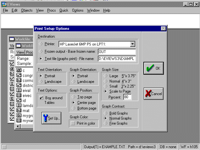
Note that ls (or LS) stands for "Least Squares" and c is a reserved word in EVIEWS that is used for the intercept term. Print the Regression Output and hand it in as a Microsoft WORD document (see below for instructions on how to do this).
Now we are going to check what happens when we eliminate the 2nd dimension DW-NOMINATE score and use a dummy variable for South/North (South = 11 states of the Confederacy plus Kentucky and Oklahoma). To do this we again use the GENR command in EVIEWS:
genr southdum=0
genr southdum=((state>=40 and state<=49) or state=51 or state=53 or state=54)*1
The first command initializes our dummy variable to zero and the second command sets it equal to one for the southern states.
Now, check to be certain that your commands correctly generated the dummy:
show state southdum
Now, run the regression:
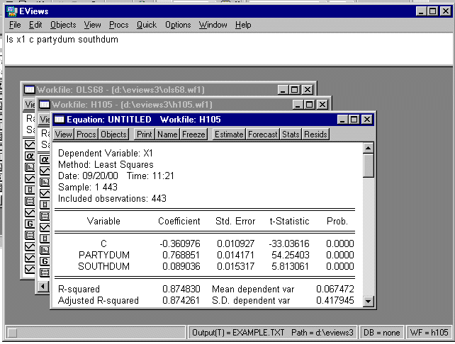
ls x1 c partydum southdum
and print the Regression Output and hand it in (for instructions, see below).
-
Our first task is to paste the
Excel spreadsheet into
Stata. To do this, start
Stata. It will look like this:
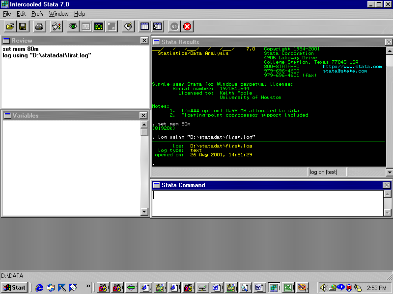
Open the data editor by clicking the icon on the toolbar and you will see this:
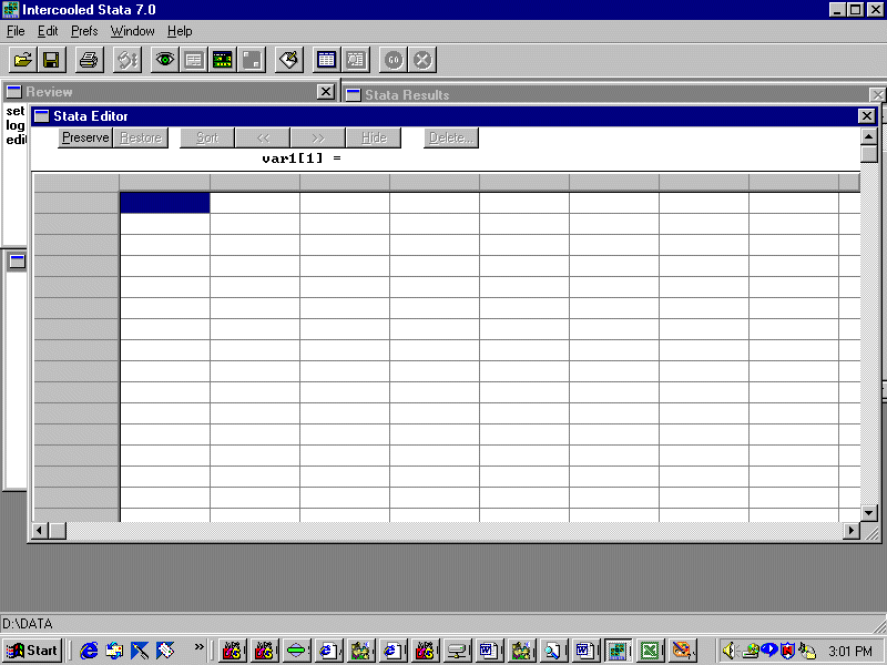
Go to Excel, put the spreadsheet on the clipboard, and then paste it into Stata. You should see this:
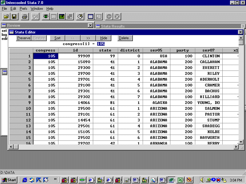
Note that the variable names are carried over from Excel.
You must now enter variable definitions into Stata. To do this, double-click on the name bar and a dialog box will come up. For example, for the variable "congress" you will see:
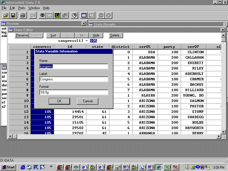
Leave the "Name:" field the same but type in the appropriate label and click "OK". For example, "Congress Number" would be an appropriate label for the variable congress. Do this for every variable (renaming ser05 and ser07 to something more descriptive is a good idea!). Now exit the editor (note that your variable descriptions now appear in Stata's variables window). Save the worksheet!
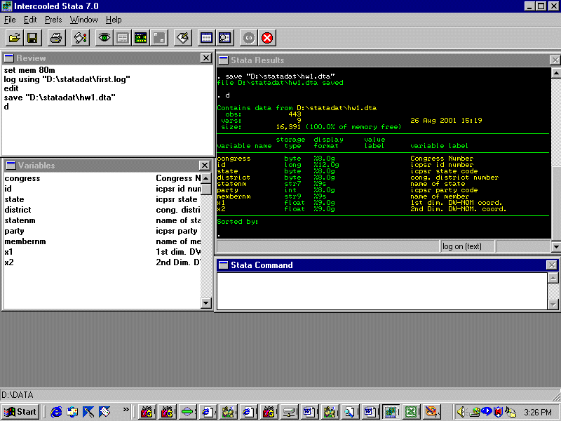
In order to preserve our output we need to open a logging file that we can in turn bring up in Epsilon. To do this click the logging file icon on the tool bar and in the dialog box select type "Log(*.log)". Now, enter the command:
d
and you will see:
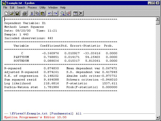
Bring your log file up in Epsilon and you will see:
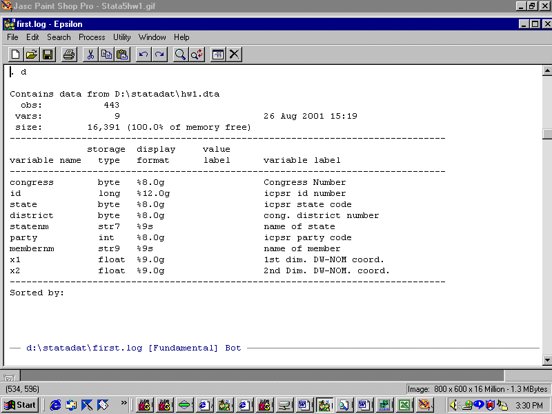
Paste the results of the d command into your homework answer (this must be a Microsoft Word document) as described below.
In Stata enter the command:
summ
and paste the results into your homework answer.
The dummy variables partydum and southdum can be created in Stata in the following manner:
generate partydum=0
replace partydum=1 if party==200
generate southdum=0
replace southdum=1 if state >= 40 & state <= 49
replace southdum=1 if state==51
replace southdum=1 if state==53
replace southdum=1 if state==54
It is a very good idea to check your work. You can do this by using the browse command in Stata which is the same as the show command in Eviews. In particular:
browse party partydum
and
browse state southdum
Open the data editor and type in definitions for partydum and southdum. Enter the d
and summ
commands and paste the results into your homework answer.
To replicate the regressions we did in Eviews, enter the following commands (note that Stata automatically puts in the intercept term -- C in Eviews):
regress x1 partydum x2
and
regress x1 partydum southdum
Paste the results into your homework answer.
