- The aim of this problem is to show you how to use the
General Purpose Optimization Routine --
optim -- in R. We are going to apply it to the
Nations Similarities data shown in Table 1.3 of Borg and Groenen that we analyzed in
Question 2 of Problem Five. Download the R
program:
 metric_mds_nations.r -- Program to
run Metric MDS on a matrix of Similarities/Dissimilarities
metric_mds_nations.r -- Program to
run Metric MDS on a matrix of Similarities/Dissimilarities#
# metric_mds_nations.r -- Does Metric MDS
#
# Wish 1971 nations similarities data
# Title: Perceived similarity of nations
#
# Description: Wish (1971) asked 18 students to rate the global
# similarity of different pairs of nations such as 'France and China' on
# a 9-point rating scale ranging from `1=very different' to `9=very
# similar'. The table shows the mean similarity ratings.
#
# Brazil 9.00 4.83 5.28 3.44 4.72 4.50 3.83 3.50 2.39 3.06 5.39 3.17
# Congo 4.83 9.00 4.56 5.00 4.00 4.83 3.33 3.39 4.00 3.39 2.39 3.50
# Cuba 5.28 4.56 9.00 5.17 4.11 4.00 3.61 2.94 5.50 5.44 3.17 5.11
# Egypt 3.44 5.00 5.17 9.00 4.78 5.83 4.67 3.83 4.39 4.39 3.33 4.28
# France 4.72 4.00 4.11 4.78 9.00 3.44 4.00 4.22 3.67 5.06 5.94 4.72
# India 4.50 4.83 4.00 5.83 3.44 9.00 4.11 4.50 4.11 4.50 4.28 4.00
# Israel 3.83 3.33 3.61 4.67 4.00 4.11 9.00 4.83 3.00 4.17 5.94 4.44
# Japan 3.50 3.39 2.94 3.83 4.22 4.50 4.83 9.00 4.17 4.61 6.06 4.28
# China 2.39 4.00 5.50 4.39 3.67 4.11 3.00 4.17 9.00 5.72 2.56 5.06
# USSR 3.06 3.39 5.44 4.39 5.06 4.50 4.17 4.61 5.72 9.00 5.00 6.67
# USA 5.39 2.39 3.17 3.33 5.94 4.28 5.94 6.06 2.56 5.00 9.00 3.56
# Yugoslavia 3.17 3.50 5.11 4.28 4.72 4.00 4.44 4.28 5.06 6.67 3.56 9.00
#
rm(list=ls(all=TRUE))
library(MASS)
library(stats)
# Optim calls a function that computes the loss function
# The user supplys the function
# &&&&&&&&&&&&&&&&&&&&&&&&&&&&&&&&&&&&&&&&&&&&&&&&&&&&&&&&&&&&&
# FUNCTION CALLED BY OPTIM(...) Below
#
# *** Calculate Log-Likelihood -- In this case simple SSE ***
# **************************************************************
fr <- function(zz){ The function is "fr" -- note that "zz" is passed into the function
xx <- zz The 12 points are stacked on top of one another in zz so that Brazil is
# zz[1] and zz[2], Congo is zz[3] and zz[4], and Yugoslavia is zz[23] and zz[24]
i <- 1
sse <- 0.0
while (i <= np) { "np" and "ndim" are defined within the program and are fixed constants
ii <- 1
while (ii <= i) {
j <- 1
dist_i_ii <- 0.0
while (j <= ndim) {
#
# Calculate distance between points
# Note the logic of selecting the points in the xx[] vector (same as zz[])
dist_i_ii <- dist_i_ii + (xx[ndim*(i-1)+j]-xx[ndim*(ii-1)+j])*(xx[ndim*(i-1)+j]-xx[ndim*(ii-1)+j])
j <- j + 1
} Here is the Loss Function -- Just simple SSE
sse <- sse + (sqrt(TT[i,ii]) - sqrt(dist_i_ii))*(sqrt(TT[i,ii]) - sqrt(dist_i_ii))
ii <- ii + 1
}
i <- i + 1
}
return(sse) The sum of squared error is returned to the optimizer
}
#
# &&&&&&&&&&&&&&&&&&&&&&&&&&&&&&&&&&&&&&&&&&&&&&&&&&&&&&&&&&&&&&&&&&&&&&&&&&&&&&&&
# The program starts here
# Read Nations Similarities Data
#
T <- matrix(scan("C:/uga_course_homework_6/nations.txt",0),ncol=12,byrow=TRUE)
#
#
np <- length(T[,1]) np is the number of rows and columns
ndim <- 2 ndim is the number of dimensions
nparam <- np*ndim nparam = number of coordinates
#
names <- NULL
names[1] <- "Brazil"
names[2] <- "Congo"
names[3] <- "Cuba"
names[4] <- "Egypt"
names[5] <- "France"
names[6] <- "India"
names[7] <- "Israel"
names[8] <- "Japan"
names[9] <- "China"
names[10] <- "USSR"
names[11] <- "USA"
names[12] <- "Yugo"
#
#
# pos -- a position specifier for the text. Values of 1, 2, 3 and 4,
# respectively indicate positions below, to the left of, above and
# to the right of the specified coordinates
#
namepos <- rep(4,np)
#namepos[1] <- 4 # Brazil
#namepos[2] <- 4 # Congo
#namepos[3] <- 4 # Cuba
#namepos[4] <- 4 # Egypt
#namepos[5] <- 4 # France
#namepos[6] <- 4 # India
#namepos[7] <- 4 # Israel
#namepos[8] <- 4 # Japan
#namepos[9] <- 4 # China
#namepos[10] <- 4 # USSR
#namepos[11] <- 4 # USA
#namepos[12] <- 4 # Yugoslavia
#
# Set Parameter Values
#
zz <- rep(0,np*ndim)
dim(zz) <- c(np*ndim,1) zz and xx are nparam length vectors used to hold the coordinates
xx <- rep(0,np*ndim)
dim(xx) <- c(np*ndim,1)
#
# Set up for Double-Centering
#
TT <- rep(0,np*np)
dim(TT) <- c(np,np)
TTT <- rep(0,np*np)
dim(TTT) <- c(np,np)
#
xrow <- NULL
xcol <- NULL
xcount <- NULL
matrixmean <- 0
#
# Transform the Matrix
#
i <- 0
while (i < np) {
i <- i + 1
xcount[i] <- i
j <- 0
while (j < np) {
j <- j + 1
#
# This is the Normal Transformation
#
TT[i,j] <- ((9 - T[i,j]))**2
#
# But the R subroutine wants simple Distances!
#
TTT[i,j] <- (9 - T[i,j])
#
}
}
#
# Call Double Center Routine From R Program
# cmdscale(....) in stats library
# The Input data are DISTANCES!!! Not Squared Distances!!
# Note that the R routine does not divide
# by -2.0
#
#
dcenter <- cmdscale(TTT,ndim, eig=FALSE,add=FALSE,x.ret=TRUE)
#
# returns double-center matrix as dcenter$x if x.ret=TRUE
#
# Do the Division by -2.0 Here
#
TTT <- (dcenter$x)/(-2.0)
#
# Perform Eigenvalue-Eigenvector Decomposition of Double-Centered Matrix
#
# ev$values are the eigenvectors
# ev$vectors are the eigenvectors
#
ev <- eigen(TTT)
# The Two Lines Below Put the Eigenvalues in a
# Diagonal Matrix -- The first one creates an
# identity matrix and the second command puts
# the singular values on the diagonal
#
Lambda <- diag(np)
diag(Lambda) <- ev$val
#
# Compute U*LAMBDA*U' for check below
#
#
XX <- ev$vec %*% Lambda %*% t(ev$vec)
#
#
# Compute Fit of decomposition -- This is just the sum of squared
# error -- Note that ssesvd should be zero!
#
#
i <- 0
j <- 0
sse <- 0
while (i < np) {
i <- i + 1
j <- 0
while (j < np) {
j <- j + 1
sse <- sse + (TTT[i,j] - XX[i,j])**2
}
}
#
# Use Eigenvectors for Starts
#
i <- 1
while (i <= np)
{
j <- 1
while (j <= ndim)
{
zz[ndim*(i-1)+j]=ev$vector[i,j] Note that the starting coordinates are stacked by dimension
j <- j +1
}
i <- i + 1
}
#
#
# *******************************************
# DO MAXIMUM LIKELIHOOD MAXIMIZATION HERE
# *******************************************
# optim is called here
model <- optim(zz,fr,hessian=TRUE,control=list(maxit=50000)) zz is the vector holding the coordinates
# Note that we pass "fr" -- the SSE routine above -- into the function
# Log-Likelihood (inverse -- optim minimizes!!)
#
logLmax <- model$value This is the minimum value it finds
#
# Parameter Estimates
#
rhomax <- model$par This is the vector of coordinates at the minimum value
#
# convergence an integer code.
# 0 indicates successful convergence.
# Error codes are
# 1 indicates that the iteration limit maxit had been reached.
# 10 indicates degeneracy of the Nelder–Mead simplex.
# 51 indicates a warning from the "L-BFGS-B" method; see component message for further details.
# 52 indicates an error from the "L-BFGS-B" method; see component message for further details.
#
nconverge <- model$convergence
#
# counts
# A two-element integer vector giving the number of calls to
# fn and gr respectively.
ncounts <- model$counts These are Important Diagnostics!! You always want to save these.
#
xhessian <- model$hessian This is the matrix of numerical 2nd derivatives
# This matrix must be full rank in order to get standard errors!!
# Check Rank of Hessian Matrix
#
evv <- eigen(xhessian)
#
# evv$values -- shows the eigenvalues Inspect the eigenvalues to see if the matrix is full rank
#
# Put Coordinates into matrix for plot purposes Note that we have been putting coordinates in a vector
# Now we transfer them into a matrix for plotting purposes
xmetric <- rep(0,np*ndim)
dim(xmetric) <- c(np,ndim)
#
i <- 1
while (i <= np)
{
j <- 1
while (j <= ndim)
{
xmetric[i,j] <- rhomax[ndim*(i-1)+j] Note the logic here
j <- j +1
}
i <- i + 1
}
#
xmax <- max(xmetric) This is the trick to get a perfect square for a
xmin <- min(xmetric) plot of our results
#
plot(xmetric[,1],xmetric[,2],type="n",asp=1,
main="",
xlab="",
ylab="",
xlim=c(xmin,xmax),ylim=c(xmin,xmax),font=2)
points(xmetric[,1],xmetric[,2],pch=16,col="red")
axis(1,font=2)
axis(2,font=2,cex=1.2)
#
# Main title
mtext("12 Nations Data",side=3,line=1.50,cex=1.2,font=2)
# x-axis title
#mtext("Liberal-Conservative",side=1,line=2.75,cex=1.2)
# y-axis title
#mtext("Region (Civil Rights)",side=2,line=2.5,cex=1.2)
#
text(xmetric[,1],xmetric[,2],names,pos=namepos,offset=00.00,col="blue",font=2)
Here is the configuration the program produces:
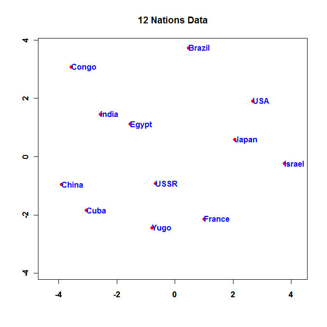
- Run the Program and turn in the resulting plot.
- Change the values in "namepos" until you have a nice looking plot with no overlapping
names and no names cut off by the margins and turn in the resulting plot.
- Report all the measures of fit -- model$value, model$convergence, and model$counts -- and report the eigenvalues
of the Hessian matrix. How many of the eigenvalues are near zero?
- Because we are working with relational data -- that is, data that can be interpreted as distances between
points -- any configuration that we estimate will be identified only up to a choice of origin and rotation.
Technically, 3 of the 24 eigenvalues of the Hessian matrix in Question (1) should be zero. The fact that we do not
get 3 zeroes indicates that
optim
has not found a true minimum of our loss function. The default optimizer in
optim is the
Nelder-Mead amoeba method which works well but
often does not get to a true minimum (maximum) when the function is highly non-linear. Fortunately, given the speed
of modern computers this is a pretty easy problem to fix. You can tell
optim to use a different optimizer
than the
Nelder-Mead amoeba method. In fact, you can use
the estimated coordinates from the
Nelder-Mead amoeba method as starts for another
method. To be certain that we get better results we are going to pass the estimated coordinates from the
Nelder-Mead amoeba method to a
Simulated Annealing Method and then pass the
estimated coordinates from the
Simulated Annealing Method to the
Broyden–Fletcher–Goldfarb–Shanno (BFGS) method.
Modify
metric_mds_nations.r as follows:
Replace:
model <- optim(zz,fr,hessian=TRUE,control=list(maxit=50000))
with:
model_nd <- optim(zz,fr,hessian=TRUE,control=list(maxit=50000))
model_sann <- optim(model_nd$par,fr,method="SANN",hessian=TRUE,control=list(maxit=50000, temp=20))
model <- optim(model_sann$par,fr,method="BFGS",hessian=TRUE)
- Report all the measures of fit for model_nd, model_sann, and model (e.g., model_nd$value, model_nd$convergence,
model_nd$counts, etc.)
- Report the eigenvalues of the Hessian matrix. How many of the eigenvalues are now near zero?
- Change the values in "namepos" until you have a nice looking plot with no overlapping
names and no names cut off by the margins and turn in the resulting plot.
- Setting one country at the origin will eliminate two of the zero eigenvalues of the Hessian matrix.
Again, because we are working with relational data -- that is, data that can be interpreted as distances between
points -- one point can be fixed at the origin without affecting the estimation of the other points because we are
trying to reproduce distances. The same distances produced by moving all the points vis a vis one another
can be generated by fixing one point and simply moving the remaining points vis a vis the fixed point. In this
problem we will fix the U.S.S.R. at the origin. Download the R
program:
metric_mds_nations_ussr.r -- Program to
run Metric MDS on a matrix of Similarities/Dissimilarities with one point fixed at the origin#
# nations_mds_nations_ussr.r -- Does Metric MDS
#
# Wish 1971 nations similarities data
# Title: Perceived similarity of nations
#
# Description: Wish (1971) asked 18 students to rate the global
# similarity of different pairs of nations such as 'France and China' on
# a 9-point rating scale ranging from `1=very different' to `9=very
# similar'. The table shows the mean similarity ratings.
#
# Brazil 9.00 4.83 5.28 3.44 4.72 4.50 3.83 3.50 2.39 3.06 5.39 3.17
# Congo 4.83 9.00 4.56 5.00 4.00 4.83 3.33 3.39 4.00 3.39 2.39 3.50
# Cuba 5.28 4.56 9.00 5.17 4.11 4.00 3.61 2.94 5.50 5.44 3.17 5.11
# Egypt 3.44 5.00 5.17 9.00 4.78 5.83 4.67 3.83 4.39 4.39 3.33 4.28
# France 4.72 4.00 4.11 4.78 9.00 3.44 4.00 4.22 3.67 5.06 5.94 4.72
# India 4.50 4.83 4.00 5.83 3.44 9.00 4.11 4.50 4.11 4.50 4.28 4.00
# Israel 3.83 3.33 3.61 4.67 4.00 4.11 9.00 4.83 3.00 4.17 5.94 4.44
# Japan 3.50 3.39 2.94 3.83 4.22 4.50 4.83 9.00 4.17 4.61 6.06 4.28
# China 2.39 4.00 5.50 4.39 3.67 4.11 3.00 4.17 9.00 5.72 2.56 5.06
# USSR 3.06 3.39 5.44 4.39 5.06 4.50 4.17 4.61 5.72 9.00 5.00 6.67
# USA 5.39 2.39 3.17 3.33 5.94 4.28 5.94 6.06 2.56 5.00 9.00 3.56
# Yugoslavia 3.17 3.50 5.11 4.28 4.72 4.00 4.44 4.28 5.06 6.67 3.56 9.00
#
rm(list=ls(all=TRUE))
library(MASS)
library(stats)
#
# &&&&&&&&&&&&&&&&&&&&&&&&&&&&&&&&&&&&&&&&&&&&&&&&&&&&&&&&&&&&&
# FUNCTION CALLED BY OPTIM(...) Below
#
# *** Calculate Log-Likelihood -- In this case simple SSE ***
# **************************************************************
fr <- function(zzz){ The function is "fr" -- note that "zzz" is passed into the function
#
xx[1:18] <- zzz[1:18] The 11 points that are being estimated are stacked on top of one another in zzz
xx[21:24] <- zzz[19:22] We transfer the 11 points to their proper position in xx[] which is length 24
xx[19:20] <- 0.0 The USSR is the 10th Country so the origin is xx[19]=xx[20]=0.0
#
i <- 1 The rest of the code in the function is the same as before
sse <- 0.0
while (i <= np) {
ii <- 1
while (ii <= i) {
j <- 1
dist_i_ii <- 0.0
while (j <= ndim) {
#
# Calculate distance between points
#
dist_i_ii <- dist_i_ii + (xx[ndim*(i-1)+j]-xx[ndim*(ii-1)+j])*(xx[ndim*(i-1)+j]-xx[ndim*(ii-1)+j])
j <- j + 1
}
sse <- sse + (sqrt(TT[i,ii]) - sqrt(dist_i_ii))*(sqrt(TT[i,ii]) - sqrt(dist_i_ii))
ii <- ii + 1
}
i <- i + 1
}
return(sse)
}
#
# &&&&&&&&&&&&&&&&&&&&&&&&&&&&&&&&&&&&&&&&&&&&&&&&&&&&&&&&&&&&&&&&&&&&&&&&&&&&&&&&
#
# Read Nations Similarities Data The code in the program is the same almost all the way down
#
T <- matrix(scan("C:/uga_course_homework_6/nations.txt",0),ncol=12,byrow=TRUE)
#
#
np <- length(T[,1])
ndim <- 2
nparam <- np*ndim
#
names <- NULL
names[1] <- "Brazil"
names[2] <- "Congo"
names[3] <- "Cuba"
names[4] <- "Egypt"
names[5] <- "France"
names[6] <- "India"
names[7] <- "Israel"
names[8] <- "Japan"
names[9] <- "China"
names[10] <- "USSR"
names[11] <- "USA"
names[12] <- "Yugo"
#
#
# pos -- a position specifier for the text. Values of 1, 2, 3 and 4,
# respectively indicate positions below, to the left of, above and
# to the right of the specified coordinates
#
namepos <- rep(4,np)
#namepos[1] <- 4 # Brazil
#namepos[2] <- 4 # Congo
#namepos[3] <- 4 # Cuba
#namepos[4] <- 4 # Egypt
#namepos[5] <- 4 # France
#namepos[6] <- 4 # India
#namepos[7] <- 4 # Israel
#namepos[8] <- 4 # Japan
#namepos[9] <- 4 # China
#namepos[10] <- 4 # USSR
#namepos[11] <- 4 # USA
#namepos[12] <- 4 # Yugoslavia
#
# Set Parameter Values
#
zz <- rep(0,np*ndim)
dim(zz) <- c(np*ndim,1)
xx <- rep(0,np*ndim)
dim(xx) <- c(np*ndim,1)
#
# Set up for Double-Centering
#
TT <- rep(0,np*np)
dim(TT) <- c(np,np)
TTT <- rep(0,np*np)
dim(TTT) <- c(np,np)
#
xrow <- NULL
xcol <- NULL
xcount <- NULL
matrixmean <- 0
#
# Transform the Matrix
#
i <- 0
while (i < np) {
i <- i + 1
xcount[i] <- i
j <- 0
while (j < np) {
j <- j + 1
#
# This is the Normal Transformation
#
TT[i,j] <- ((9 - T[i,j]))**2
#
# But the R subroutine wants simple Distances!
#
TTT[i,j] <- (9 - T[i,j])
#
}
}
#
# Call Double Center Routine From R Program
# cmdscale(....) in stats library
# The Input data are DISTANCES!!! Not Squared Distances!!
# Note that the R routine does not divide
# by -2.0
#
#
dcenter <- cmdscale(TTT,ndim, eig=FALSE,add=FALSE,x.ret=TRUE)
#
# returns double-center matrix as dcenter$x if x.ret=TRUE
#
# Do the Division by -2.0 Here
#
TTT <- (dcenter$x)/(-2.0)
#
# Perform Eigenvalue-Eigenvector Decomposition of Double-Centered Matrix
#
# ev$values are the eigenvectors
# ev$vectors are the eigenvectors
#
ev <- eigen(TTT)
# The Two Lines Below Put the Eigenvalues in a
# Diagonal Matrix -- The first one creates an
# identity matrix and the second command puts
# the singular values on the diagonal
#
Lambda <- diag(np)
diag(Lambda) <- ev$val
#
# Compute U*LAMBDA*U' for check below
#
#
XX <- ev$vec %*% Lambda %*% t(ev$vec)
#
#
# Compute Fit of decomposition -- This is just the sum of squared
# error -- Note that ssesvd should be zero!
#
#
i <- 0
j <- 0
sse <- 0
while (i < np) {
i <- i + 1
j <- 0
while (j < np) {
j <- j + 1
sse <- sse + (TTT[i,j] - XX[i,j])**2
}
}
#
# Use Eigenvectors for Starts
#
i <- 1
while (i <= np)
{
j <- 1
while (j <= ndim)
{
zz[ndim*(i-1)+j]=ev$vector[i,j]
j <- j +1
}
i <- i + 1
}
#
# CONSTRAIN USSR TO THE ORIGIN Now the code is different -- Here we do the reverse of what we did in the function
# We transfer the coordinates for the countries except the USSR into zzz[]
zzz <- rep(0,(np-1)*ndim) zzz[] is length 22 -- So optim estimates 22 parameters using function "fr" above
dim(zzz) <- c((np-1)*ndim,1)
zzz[1:18] <- zz[1:18]
zzz[19:22] <- zz[21:24]
#
# *******************************************
# DO MAXIMUM LIKELIHOOD MAXIMIZATION HERE
# *******************************************
#
model_nd <- optim(zzz,fr,hessian=TRUE,control=list(maxit=50000))
model_sann <- optim(model_nd$par,fr,method="SANN",hessian=TRUE,control=list(maxit=50000, temp=20))
model <- optim(model_sann$par,fr,method="BFGS",hessian=TRUE)
#
# Log-Likelihood (inverse -- optim minimizes!!)
#
logLmax <- model$value
#
# Parameter Estimates
#
rhomax <- model$par
#
# convergence an integer code.
# 0 indicates successful convergence.
# Error codes are
# 1 indicates that the iteration limit maxit had been reached.
# 10 indicates degeneracy of the Nelder–Mead simplex.
# 51 indicates a warning from the "L-BFGS-B" method; see component message for further details.
# 52 indicates an error from the "L-BFGS-B" method; see component message for further details.
#
nconverge <- model$convergence
#
# counts
# A two-element integer vector giving the number of calls to
# fn and gr respectively.
#
ncounts <- model$counts
#
xhessian <- model$hessian
#
# Check Rank of Hessian Matrix
#
evv <- eigen(xhessian)
#
# evv$values -- shows the eigenvalues
#
# Put Coordinates into matrix for plot purposes Things get tricky here because we have to do some bookkeeping
# to keep track of the fact that we have set the USSR at the origin
xmetric <- rep(0,np*ndim)
dim(xmetric) <- c(np,ndim)
#
i <- 1
kk <- 1
while (i <= np)
{
j <- 1
while (j <= ndim)
{ Note the counter "kk" -- it increments from 1 to 11 skipping the USSR
if(i != 10){
xmetric[i,j] <- rhomax[ndim*(kk-1)+j]
} When we get to the USSR we stick 0.0's in xmetric[,]
if(i==10)xmetric[i,j]=0.0
j <- j +1
} kk is only incremented when i is not equal to 10 -- the USSR
if(i!= 10)kk <- kk + 1
i <- i + 1
}
#
xmax <- max(xmetric)
xmin <- min(xmetric)
#
plot(xmetric[,1],xmetric[,2],type="n",asp=1,
main="",
xlab="",
ylab="",
xlim=c(xmin,xmax),ylim=c(xmin,xmax),font=2)
points(xmetric[,1],xmetric[,2],pch=16,col="red")
axis(1,font=2)
axis(2,font=2,cex=1.2)
#
# Main title
mtext("12 Nations Data",side=3,line=1.50,cex=1.2,font=2)
# x-axis title
#mtext("Liberal-Conservative",side=1,line=2.75,cex=1.2)
# y-axis title
#mtext("Region (Civil Rights)",side=2,line=2.5,cex=1.2)
#
text(xmetric[,1],xmetric[,2],names,pos=namepos,offset=00.00,col="blue",font=2)
- Report all the measures of fit for model_nd, model_sann, and model (e.g., model_nd$value, model_nd$convergence,
model_nd$counts, etc.)
- Report the eigenvalues of the Hessian matrix. How many of the eigenvalues are now near zero?
- Change the values in "namepos" until you have a nice looking plot with no overlapping
names and no names cut off by the margins and turn in the resulting plot.