What we are going to do is use a program to simulate this process and numerically compute the expected value of e-kd for 40 values of the true distance (from 0 to 2) between the true locations of the stimuli.
Use the following R program below to do this experiment:
Here is what the program looks like:
#
#
#  normal_2.r -- Test of Shepard_Ennis_Nofosky model of Stimulus
#                Comparison
#
#   Exemplars have bivariate normal distributions.  One point is
#      drawn from each distribution and the distance computed.
#      This distance is then exponentiated -- exp(-d) -- and
#      this process is repeated m times to get a E[exp(-d)].
#
#   Note that when STDDEVX is set very low then this is equivalent
#      to a legislator's ideal point so that the stimulus comparison
#      is between the ideal point and the momentary draw from the
#      Exemplar distribution.
#
#  Set Means and Standard Deviations of Two Bivariate Normal Distributions
#
#  Remove all objects just to be safe
#
rm(list=ls(all=TRUE))
#
STDDEVX <- .001                  Initialize Means and Standard
STDDEVY <- .4                     Deviations of the Two Normal Distributions
XMEAN <- 0
YMEAN <- 0
#
#  Set Number of Draws to Get Expected Value
#
m <- 10000
#
#  Set Number of Points
#
n <- 40
#
#  Set Increment for Distance Between Two Bivariate Normal Distributions
#
XINC <- 0.05                    Note that n*XINC = 2.0
#
x <- NULL                       Initialize vectors
y <- NULL
z <- NULL
xdotval <- NULL
ydotval <- NULL
zdotval <- NULL
iii <- 0
while (iii <= n) {              ****Start of Outer Loop -- it Executes Until y has n=40 Entries
   x <- 0
   i <- 0
   iii <- iii + 1
   while (i <= m) {             ****Start of Inner Loop -- it Executes m=10000 Times
#
#  Draw points from the two bivariate normal distributions
#              Draw two numbers randomly from Normal Distribution with Mean XMEAN and stnd. dev. of STDDEVX and put them in the vector xdotval
       xdotval <- c(rnorm(2,XMEAN,STDDEVX))
       ydotval <- c(rnorm(2,YMEAN,STDDEVY))
#              Draw two numbers randomly from Normal Distribution with Mean YMEAN and stnd. dev. of STDDEVY and put them in the vector ydotval
#  Compute distance Between two randomly drawn points
#              Calculate Euclidean Distance Between xdotval and ydotval
       zdotval <- sqrt((xdotval[1]-ydotval[1])**2 + (xdotval[2]-ydotval[2])**2)
#
#  Exponentiate the distance
#
       zdotval <- exp(-zdotval)
#
#  Compute Expected Value
#
       x <- x + zdotval/m  Store exp(-d) in x -- note the division by m so that x will contain
       i <- i + 1             the mean after m=10000 trials
   }                       ****End of Inner Loop
#
#  Store Expected Value and Distance Between Means of Two Distributions
#
    y[iii] <- x
    z[iii] <- sqrt(2*YMEAN^2)
    YMEAN <- YMEAN + XINC      Increment YMEAN by .05
}                              ****End of Outer Loop
#
#  The type="n" tells R to not display anything
#
plot(z,y,xlim=c(0,3),ylim=c(0,.7),type="n",
     main="",
     xlab="",
     ylab="",font=2)
#
#  Another Way of Doing the Title
#
title(main="Test of Shepard-Ennis-Nofosky, .001, .4\nTest of Ideal Point vs. Outcome Model")
# Main title
mtext("Test of Shepard-Ennis-Nofosky, .001, .4\nTest of Ideal Point vs. Outcome Model",side=3,line=1.00,cex=1.2,font=2)
# x-axis title
mtext("True Distance Between Stimuli",side=1,line=2.75,font=2,cex=1.2)
# y-axis title
mtext("Expected Value of Observed Similarity",side=2,line=2.75,font=2,cex=1.2)
##
#  An Alternative Way to Plot the Points and the Lines
#
points(z,y,pch=16,col="blue",font=2)
lines(z,y,lty=1,lwd=2,font=2,col="red")
#
The program will produce a graph that looks similar to this: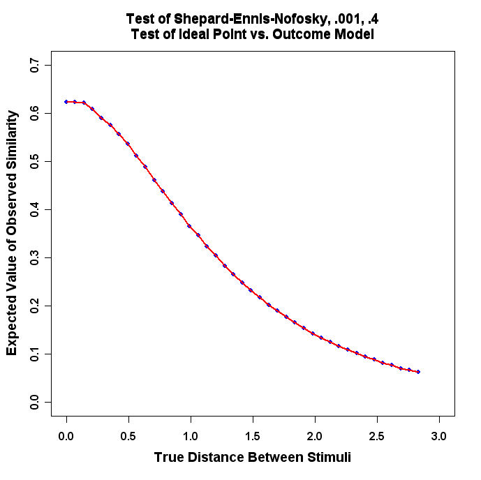
- Run the Program and turn in the resulting plot.
- Use Epsilon to change STDDEVX and
STDDEVY
in Shepard-Ennis-Nofosky_1.R, re-load it into R, and produce
a plot like the above. For example, change STDDEVX to .1 and STDDEVY
to .4 and re-run the program. Change the "title" each time to reflect the
different values! Pick 3 pairs of
reasonable values of STDDEVX and STDDEVY and produce plots for
each experiment.
#
# double_center_drive_data.r -- Double-Center Program
#
# Data Must Be Transformed to Squared Distances Below
#
# ATLANTA      0000 2340 1084  715  481  826 1519 2252  662  641 2450
# BOISE        2340 0000 2797 1789 2018 1661  891  908 2974 2480  680
# BOSTON       1084 2797 0000  976  853 1868 2008 3130 1547  443 3160
# CHICAGO       715 1789  976 0000  301  936 1017 2189 1386  696 2200
# CINCINNATI    481 2018  853  301 0000  988 1245 2292 1143  498 2330
# DALLAS        826 1661 1868  936  988 0000  797 1431 1394 1414 1720
# DENVER       1519  891 2008 1017 1245  797 0000 1189 2126 1707 1290
# LOS ANGELES  2252  908 3130 2189 2292 1431 1189 0000 2885 2754  370
# MIAMI         662 2974 1547 1386 1143 1394 2126 2885 0000 1096 3110
# WASHINGTON    641 2480  443  696  498 1414 1707 2754 1096 0000 2870
# CASBS        2450  680 3160 2200 2330 1720 1290  370 3110 2870 0000
#
#  Remove all objects just to be safe
#
rm(list=ls(all=TRUE))
#
library(MASS)
library(stats)
#
#
T <- matrix(scan("C:/ucsd_course/drive2.txt",0),ncol=11,byrow=TRUE)
#
nrow <- length(T[,1])
ncol <- length(T[1,])
#               Another way of entering names -- Note the space after the name
names <- c("Atlanta ","Boise ","Boston ","Chicago ","Cincinnati ","Dallas ","Denver ",
           "Los Angeles ","Miami ","Washington ","CASBS ")
#
# pos -- a position specifier for the text. Values of 1, 2, 3 and 4,
# respectively indicate positions below, to the left of, above and
# to the right of the specified coordinates
#
namepos <- rep(2,nrow)
#
TT <- rep(0,nrow*ncol)
dim(TT) <- c(nrow,ncol)
TTT <- rep(0,nrow*ncol)
dim(TTT) <- c(nrow,ncol)
#
xrow <- NULL
xcol <- NULL
xcount <- NULL
matrixmean <- 0
matrixmean2 <- 0
#
# Transform the Matrix
#
i <- 0
while (i < nrow) {
  i <- i + 1
  xcount[i] <- i          Ignore -- Just a diagnostic
  j <- 0
  while (j < ncol) {
     j <- j + 1
#
#  Square the Driving Distances
#
     TT[i,j] <- (T[i,j]/1000)**2  Note the division by 1000 for scale purposes
#
  }
}
#
#  Put it Back in T
#
T <- TT
TTT <- sqrt(TT)    This creates distances -- see below
#
#
#  Call Double Center Routine From R Program
#     cmdscale(....) in stats library
#     The Input data are DISTANCES!!!  Not Squared Distances!!
#     Note that the R routine does not divide
#     by -2.0
#
ndim <- 2
#
dcenter <- cmdscale(TTT,ndim, eig=FALSE,add=FALSE,x.ret=TRUE)
#
#  returns double-center matrix as dcenter$x if x.ret=TRUE
#
#  Do the Division by -2.0 Here
#
TTT <- (dcenter$x)/(-2.0)       Here is the Double-Centered Matrix
#
#
#  Below is the old Long Method of Double-Centering
#
# Compute Row and Column Means
#
i <- 0
while (i < nrow) {
  i <- i + 1
  xrow[i] <- mean(T[i,])
}
i <- 0
while (i < ncol) {
  i <- i + 1
  xcol[i] <- mean(T[,i])
}
matrixmean <- mean(xcol)
matrixmean2 <- mean(xrow)
#
# Double-Center the Matrix Using old Long Method
#  Compute comparison as safety check
#
i <- 0
while (i < nrow) {
  i <- i + 1
  j <- 0
  while (j < ncol) {
     j <- j + 1
     TT[i,j] <- (T[i,j]-xrow[i]-xcol[j]+matrixmean)/(-2)  This is the Double-Center Operation
  }
}
#
#  Run some checks to make sure everything is correct
#
xcheck <- sum(abs(TT-TTT))   This checks to see if both methods are the same numerically
#
#
#  Perform Eigenvalue-Eigenvector Decomposition of Double-Centered Matrix
#
ev <- eigen(TT)
#
#  Find Point furthest from Center of Space
#
aaa <- sqrt(max((abs(ev$vec[,1]))**2 + (abs(ev$vec[,2]))**2))  These two commands do the same thing
bbb <- sqrt(max(((ev$vec[,1]))**2 + ((ev$vec[,2]))**2))
#
#  Weight the Eigenvectors to Scale Space to Unit Circle
#
torgerson1 <- ev$vec[,1]*(1/aaa)*sqrt(ev$val[1])
torgerson2 <- -ev$vec[,2]*(1/aaa)*sqrt(ev$val[2])  Note the Sign Flip
#
plot(torgerson1,torgerson2,type="n",asp=1,
       main="",
       xlab="",
       ylab="",
       xlim=c(-3.0,3.0),ylim=c(-3.0,3.0),font=2)
points(torgerson1,torgerson2,pch=16,col="red",font=2)
text(torgerson1,torgerson2,names,pos=namepos,offset=0.2,col="blue",font=2)  Experiment with the offset value
#
#
# Main title
mtext("Double-Centered Driving Distance Matrix \n Torgerson Coordinates",side=3,line=1.25,cex=1.5,font=2)
# x-axis title
mtext("West    ---    East",side=1,line=2.75,cex=1.2,font=2)
# y-axis title
mtext("South    ---    North",side=2,line=2.5,cex=1.2,font=2)
#
The program will produce a graph that looks similar to this: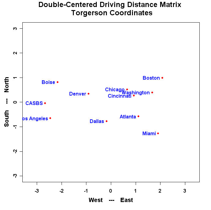
- Run the Program and turn in the resulting plot.
- Change the values in "namepos" until you have a nice looking plot with no overlapping
names and no names cut off by the margins and turn in the resulting plot.
- Use Epsilon to add a 12th city (you will have
to get a driving atlas to do this) to Drive2.txt and call the matrix Drive3.txt.
Modify the R program to read and plot the 12 by 12 driving
distance matrix. Turn in Drive3.txt, the resulting plot, and the modified
R program.
#
#
# double_center_color_circle.r -- Double-Center Program
#
# Data Must Be Transformed to Squared Distances Below
#
#      **************** The Eckman Color Data *****************
#
# 434 INDIGO        100  86  42  42  18   6   7   4   2   7   9  12  13  16
# 445 BLUE           86 100  50  44  22   9   7   7   2   4   7  11  13  14
# 465                42  50 100  81  47  17  10   8   2   1   2   1   5   3
# 472 BLUE-GREEN     42  44  81 100  54  25  10   9   2   1   0   1   2   4
# 490                18  22  47  54 100  61  31  26   7   2   2   1   2   0
# 504 GREEN           6   9  17  25  61 100  62  45  14   8   2   2   2   1
# 537                 7   7  10  10  31  62 100  73  22  14   5   2   2   0
# 555 YELLOW-GREEN    4   7   8   9  26  45  73 100  33  19   4   3   2   2
# 584                 2   2   2   2   7  14  22  33 100  58  37  27  20  23
# 600 YELLOW          7   4   1   1   2   8  14  19  58 100  74  50  41  28
# 610                 9   7   2   0   2   2   5   4  37  74 100  76  62  55
# 628 ORANGE-YELLOW  12  11   1   1   1   2   2   3  27  50  76 100  85  68
# 651 ORANGE         13  13   5   2   2   2   2   2  20  41  62  85 100  76
# 674 RED            16  14   3   4   0   1   0   2  23  28  55  68  76 100
#
#
#  Remove all objects just to be safe
#
rm(list=ls(all=TRUE))
#
library(MASS)
library(stats)
#
#
rcx.file <- "c:/ucsd_course/color_circle.txt"
#
# Standard fields and their widths
#
rcx.fields <- c("colorname","x1","x2","x3","x4","x5",
                   "x6","x7","x8","x9","x10","x11","x12","x13","x14")
rcx.fieldWidths <- c(18,4,4,4,4,4,4,4,4,4,4,4,4,4,4)
#
# Read the vote data from fwf
#
U <- read.fwf(file=rcx.file,widths=rcx.fieldWidths,as.is=TRUE,col.names=rcx.fields)
dim(U)
ncolU <- length(U[1,])   Note the "trick" I used here
T <- U[,2:ncolU]           The 1st column of U has the color names
#
#
nrow <- length(T[,1])
ncol <- length(T[1,])
#           Even though I have the color names in U this is more convenient
#             because there are no leading or trailing blanks
names <- c("434 Indigo","445 Blue","465","472 Blue-Green","490","504 Green","537",
           "555 Yellow-Green","584","600 Yellow","610","628 Orange-Yellow",
           "651 Orange","674 Red")
#
# pos -- a position specifier for the text. Values of 1, 2, 3 and 4,
# respectively indicate positions below, to the left of, above and
# to the right of the specified coordinates
#
namepos <- rep(2,nrow)
#
TT <- rep(0,nrow*ncol)
dim(TT) <- c(nrow,ncol)
TTT <- rep(0,nrow*ncol)
dim(TTT) <- c(nrow,ncol)
#
xrow <- NULL
xcol <- NULL
xcount <- NULL
matrixmean <- 0
matrixmean2 <- 0
#
# Transform the Matrix
#
i <- 0
while (i < nrow) {
  i <- i + 1
  xcount[i] <- i
  j <- 0
  while (j < ncol) {
     j <- j + 1
#
#  Transform the Color "Agreement Scores" into Distances
#
     TT[i,j] <- ((100-T[i,j])/50)**2   Note the Transformation from a 100 to 0 scale
#                                        to a 0 to 4 (squared distance) scale
  }
}
#
#  Put it Back in T
#
T <- TT
TTT <- sqrt(TT)
#
#
#  Call Double Center Routine From R Program
#     cmdscale(....) in stats library
#     The Input data are DISTANCES!!!  Not Squared Distances!!
#     Note that the R routine does not divide
#     by -2.0
#
ndim <- 2
#
dcenter <- cmdscale(TTT,ndim, eig=FALSE,add=FALSE,x.ret=TRUE)
#
#  returns double-center matrix as dcenter$x if x.ret=TRUE
#
#  Do the Division by -2.0 Here
#
TTT <- (dcenter$x)/(-2.0)
#
#
#  Below is the old Long Method of Double-Centering
#
# Compute Row and Column Means
#
i <- 0
while (i < nrow) {
  i <- i + 1
  xrow[i] <- mean(T[i,])
}
i <- 0
while (i < ncol) {
  i <- i + 1
  xcol[i] <- mean(T[,i])
}
matrixmean <- mean(xcol)
matrixmean2 <- mean(xrow)
#
# Double-Center the Matrix Using old Long Method
#  Compute comparison as safety check
#
i <- 0
while (i < nrow) {
  i <- i + 1
  j <- 0
  while (j < ncol) {
     j <- j + 1
     TT[i,j] <- (T[i,j]-xrow[i]-xcol[j]+matrixmean)/(-2)
  }
}
#
#  Run some checks to make sure everything is correct
#
xcheck <- sum(abs(TT-TTT))
#
#
#  Perform Eigenvalue-Eigenvector Decomposition of Double-Centered Matrix
#
ev <- eigen(TT)
#
#  Find Point furthest from Center of Space
#
aaa <- sqrt(max((abs(ev$vec[,1]))**2 + (abs(ev$vec[,2]))**2))
bbb <- sqrt(max(((ev$vec[,1]))**2 + ((ev$vec[,2]))**2))
#
#  Weight the Eigenvectors to Scale Space to Unit Circle
#
torgerson1 <- ev$vec[,1]*(1/aaa)*sqrt(ev$val[1])
torgerson2 <- -ev$vec[,2]*(1/aaa)*sqrt(ev$val[2])
#
plot(torgerson1,torgerson2,type="n",asp=1,
       main="",
       xlab="",
       ylab="",
       xlim=c(-3.0,3.0),ylim=c(-3.0,3.0),font=2)
points(torgerson1,torgerson2,pch=16,col="red",font=2)
text(torgerson1,torgerson2,names,pos=namepos,offset=0.2,col="blue",font=2)
#
#
# Main title
mtext("The Color Circle \n Torgerson Coordinates",side=3,line=1.25,cex=1.5,font=2)
# x-axis title
mtext("",side=1,line=2.75,cex=1.2,font=2)
# y-axis title
mtext("",side=2,line=2.5,cex=1.2,font=2)
#
Run the program and you should see something like this: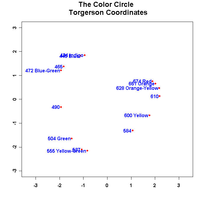
- Run the program and turn in this figure.
- Change the values in "namepos" until you have a nice looking plot with no overlapping
names and no names cut off by the margins and turn in the resulting plot. Use the offset
parameter in the text command to space the names away from the points. Also
flip the dimensions as appropriate so that the configuration matches the one
in Borg and Goenen!
- Check out:
Color Circle in Color
Use the colors() command in R to find the corresponding colors and then use the text command to color the label for the corresponding point; e.g.,
text(torgerson1[10],torgerson2[10],"Yellow",pos=4,col="yellow",font=2)
You will have to override the labeling command in the double-center program to do this. Turn in the plot (hard copy in B/W and e-mail it to me so I can see it!) and the listing of your R program.
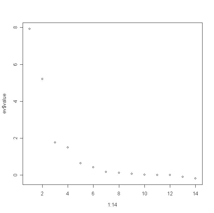
- Plot the eigenvalues that are stored in ev$value. The simplest plot is to use the command at the
R prompt:
plot(1:14,ev$value)
and you will get the following really lame graph:
Turn this into a nicer graph. To do this, check out the R code for Figure 5.4 of my book which is posted on my website at:
Chapter 5 Page
Turn in a final graph and a listing of the R code you use to create it.
 434_INDIGO        100  86  42  42  18   6   7   4   2   7   9  12  13  16
 445_BLUE           86 100  50  44  22   9   7   7   2   4   7  11  13  14
 465                42  50 100  81  47  17  10   8   2   1   2   1   5   3
 472_BLUE-GREEN     42  44  81 100  54  25  10   9   2   1   0   1   2   4
 490                18  22  47  54 100  61  31  26   7   2   2   1   2   0
 504_GREEN           6   9  17  25  61 100  62  45  14   8   2   2   2   1
 537                 7   7  10  10  31  62 100  73  22  14   5   2   2   0
 555_YELLOW-GREEN    4   7   8   9  26  45  73 100  33  19   4   3   2   2
 584                 2   2   2   2   7  14  22  33 100  58  37  27  20  23
 600_YELLOW          7   4   1   1   2   8  14  19  58 100  74  50  41  28
 610                 9   7   2   0   2   2   5   4  37  74 100  76  62  55
 628_ORANGE-YELLOW  12  11   1   1   1   2   2   3  27  50  76 100  85  68
 651_ORANGE         13  13   5   2   2   2   2   2  20  41  62  85 100  76
 674_RED            16  14   3   4   0   1   0   2  23  28  55  68  76 100
then change the format statement to:
(18X,101F4.0)
Be sure to change the missing values parameter to a negative number because there are some zeroes in the matrix. Your KYST file should look like the following:
TORSCA
PRE-ITERATIONS=3
DIMMAX=3,DIMMIN=1
PRINT HISTORY,PRINT DISTANCES
COORDINATES=ROTATE
ITERATIONS=50
REGRESSION=DESCENDING
DATA,LOWERHALFMATRIX,DIAGONAL=PRESENT,CUTOFF=-.01
EKMAN'S COLOR DATA EXAMPLE
 14  1  1
(18X,101F4.0)
****the color data****
COMPUTE
STOP
- Run all tables from 3 to 1 dimensions, report the Stress values, and
use R to graph the results for each table in two
dimensions.
- Produce Shepard Diagrams for each two dimensional solution in the same
format as Homework 2.