LEGACY CONTENT. If you are looking for Voteview.com, PLEASE CLICK HERE

This site is an archived version of Voteview.com archived from University of Georgia on May 23, 2017. This point-in-time capture includes all files publicly linked on Voteview.com at that time. We provide access to this content as a service to ensure that past users of Voteview.com have access to historical files. This content will remain online until at least January 1st, 2018. UCLA provides no warranty or guarantee of access to these files.

"Common Space" DW-NOMINATE Scores With Bootstrapped Standard Errors
(Joint House and Senate Scaling)

Royce Carroll, Jeff Lewis, James Lo, Nolan McCarty, Keith Poole, and Howard Rosenthal

Updated 2 September 2015

This is the fifth release of Common Space DW-NOMINATE scores for the House and Senate. The House and Senate were scaled as if they were one legislature using the 650 Legislators who served in both the House and Senate as "glue" (bridge observations). That is, we estimated a single ideal point for each member of Congress based upon his/her entire record of service in Congress. In the Poole-Rosenthal framework we used the Constant model so that each unique legislator has the same ideal point throughout his or her career. After the download links we show some comparisons of these Common Space scores with our regular DW-NOMINATE Scores for the House and Senate.

These new scores for the 1^st to the 113^th Congresses (1789 - 2014) contain parametric bootstrapped standard errors. For an explanation of the basic theory of the parametric bootstrap see:

Political Analysis

Jeffrey B. Lewis

Keith T. Poole

Political Analysis

This research was made possible by NSF Grant 0611880 to Jeffrey B. Lewis
Keith T. Poole, and Howard Rosenthal. This work was also supported in part by the Rice Terascale Cluster funded by NSF under Grant EIA-0216467, and a partnership between Rice University, Intel, and HP. We thank the National Science Foundation and the San Diego Supercomputer Center for their support.

There were a total of 102,806 roll calls of which 92,182 were scalable. The number of unique legislators was 11,976 producing a total of 16,980,265 choices. In the scaling, the second dimension weight is 0.4113 and the Beta parameter (proportional to 1/s where s is the standard deviation of the error) is 7.8334. The correct classification is 87.21 percent with an APRE of 0.6215 and a geometric mean probability of 0.7533.

In order to calculate distances from these Common Space DW-NOMINATE scores you must multiply the second dimension by the weight parameter. To calculate the choice probabilities you must apply both the second dimension weight and the Beta parameter. Use the Yea and Nay outcome coordinates with considerable caution because, as we explain in Congress: A Political Economic History of Roll Call Voting, they are poorly identified. However, the cutting line is identified and can be used safely.

Please note that these files contain scores for most Presidents. For Presidents prior to Eisenhower these are based on roll calls corresponding to Presidential requests. These roll calls were compiled by an NSF project headed by Elaine Swift ( Study No. 3371, Database of Congressional Historical Statistics, 1789-1989). Many of these scores are based upon a small number of roll calls so use them with caution!

In the files below the House Coordinates for each Congress are stacked on top of the Senate coordinates. If you have questions or need help with these files please send us e-mail at jblewis@ucla.edu (Jeff Lewis) or ktpoole@uga.edu (Keith Poole).

The format of the legislator files is:


 1.  Congress Number
 2.  ICPSR ID Number:  5 digit code assigned by the ICPSR as
                       corrected by Howard Rosenthal and myself.
 3.  State Code:  2 digit ICPSR State Code.
 4.  Congressional District Number (0 if Senate or President)
 5.  State Name
 6.  Party Code:  100 = Dem., 200 = Repub. (See PARTY3.DAT)
 7.  Name
 8.  1st Dimension Coordinate
 9.  2nd Dimension Coordinate
10.  1st Dimension Bootstrapped Standard Error  
11.  2nd Dimension Bootstrapped Standard Error  
12.  Correlation Between 1st and 2nd Dimension Bootstrapped Estimates
13.  Log-Likelihood
14.  Number of Votes
15.  Number of Classification Errors
16.  Geometric Mean Probability

The format of the roll call files is:

 1.  Congress Number
 2.  Roll Call Number
 3.  "H" if House, "S" if Senate
 4.  Number of Yeas
 5.  Number of Nays
 6.  Month of Roll Call
 7.  Day of Roll Call
 8.  Year of Roll Call
 9.  Number Correctly Classified
10.  Predicted Yea/Actual Yea
11.  Predicted Yea/Actual Nay
12.  Predicted Nay/Actual Yea
13.  Predicted Nay/Actual Nay
14.  Proportion Correctly Classified (#9 divided by #4 + #5)
15.  Proportional Reduction in Error (PRE) -- (Min. on RC - Error)/Min. on RC
16.  Geometric Mean Probability
17.  Spread on 1st Dimension    -- if the roll call was not scaled, there
18.  Midpoint on 1st Dimension  -- are 0.000's in all four fields
19.  Spread on 2nd Dimension    --
20.  Midpoint on 2nd Dimension  --

Legislator Estimates 1^st to 113^th Houses and Senates (Text File, 46,506 lines)
Legislator Estimates 1^st to 113^th Houses and Senates (Stata 14 File, 46,506 lines)
Legislator Estimates 1^st to 113^th Houses and Senates (Stata 12 File, 46,506 lines)
Legislator Estimates 1^st to 113^th Houses and Senates (Eviews File, 46,506 lines)
Legislator Estimates 1^st to 113^th Houses and Senates (Excel File, 46,506 lines)

Roll Call Estimates 1^st to 113^th Houses and Senates (Text File, 102,806 lines)
Roll Call Estimates 1^st to 113^th Houses and Senates (Stata 13 File, 102,806 lines)
Roll Call Estimates 1^st to 113^th Houses and Senates (Stata 12 File, 102,806 lines)
Roll Call Estimates 1^st to 113^th Houses and Senates (Eviews File, 102,806 lines)
Roll Call Estimates 1^st to 113^th Houses and Senates (Excel File, 102,806 lines)

A Comparison of the "Common Space" DW-NOMINATE Scores With the Separate House and Senate 2-Dimensional Linear DW-NOMINATE Scores

The Joint Scaling of the House and Senate utilizes the 2-dimensional constant model developed by Poole and Rosenthal in which each legislator has a single ideal point throughout his or her career. In contrast, the standard DW-NOMINATE scores use the 2-dimensional linear model in which a legislator is allowed to move on a straight line throughout his or her career. These models are discussed in detail in:

Keith T. Poole and Howard Rosenthal. 1997. Congress: A Political-Economic History of Roll Call Voting. New York: Oxford University Press.
Keith T. Poole and Howard Rosenthal. 2007. Ideology and Congress. Piscataway, N.J.: Transaction Press.
Keith T. Poole. 2005. Spatial Models of Parliamentary Voting. New York: Cambridge University Press.

In the table below we show the fit statistics for the Joint Scaling and the separate scalings for the House and Senate posted on the DW-NOMINATE Scores Page.

                        Joint Scaling    House Only   Senate Only
                           (2-D Const.)  (2-D Lin.)   (2-D Lin.)
....................................................................
Correct Classification        87.2100      87.7670      86.1230
APRE                           0.6215       0.6377       0.5906
GMP                            0.7533       0.7608       0.7440
Beta                           7.8334       7.8332      10.1105
Weight-2nd                     0.4113       0.3988       0.5638
                          ..........................................
Unique Legisislators           11,976       10,731        1,895
Total Roll Calls              102,806       53,530       49,276
Scalable Roll Calls            92,182       46,865       45,317
Total Choices              16,980,265   13,879,366    3,100,516

The fit of the Joint Scaling is a half percentage point below the House fit but better than the Senate fit. This reflects the fact that the House fit is better than the Senate fit and the number of unique members in the House is more than five times the number of unique members of the Senate. Consequently, when the chambers are combined it is not surprising that the larger number of House members -- even with the constraint of the constant model -- will drive the fit.

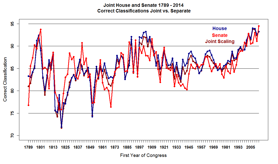
Below is a graph of the correct classifications for these three scalings. The pattern of the classifications is essentially the same as that shown in Figure 3.1 of Ideology and Congress. The correct classification of the joint scaling closely tracks that for the separate House DW-NOMINATE scaling. The Pearson correlation between the two is 0.988. The corresponding correlation between the joint scaling and the separate Senate DW-NOMINATE scaling is 0.807. However, the correlation between the correct classifications for the Senates within the joint scaling and the separate Senate DW-NOMINATE scaling is 0.986. The corresponding correlation between the correct classifications for the Houses within the joint scaling and the separate House DW-NOMINATE scaling is 0.998. What these correlations show is that, although constraining the members of Congress to having a single ideal point throughout their careers, the patterns of overall chamber classifications are almost exactly reproduced even though on average the classifications of the joint model are lower.

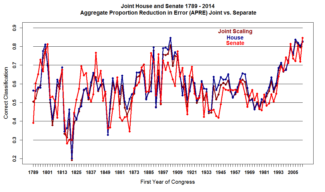
The graph below shows the Aggregate Proportional Reduction in Error (APRE). The APRE controls for the margins of the roll calls and is defined as (TOTAL MINORITY VOTES - CLASSIFICATION ERROR)/TOTAL MINORITY VOTES. Hence, if the spatial model simply predicts the majority number on each roll call the classification error will equal the total of the minority votes and APRE will be zero. This controls for the fact that if you have a large number of lopsided roll calls you can have a high rate of classification. The APRE statistic accounts for this by making the benchmark correctly classifying the minority votes (so to speak).

Note that since the 1970s APRE has climbed rapidly and is about 0.85 while the average majority margin on the roll calls in the two chambers has been between 70% to 65%. Most roll call votes in the current unidimensional era are all of one party plus the closest wing of the opposite party versus the remainder of the opposite party. This is why the APRE and the Correct Classification have risen so sharply.

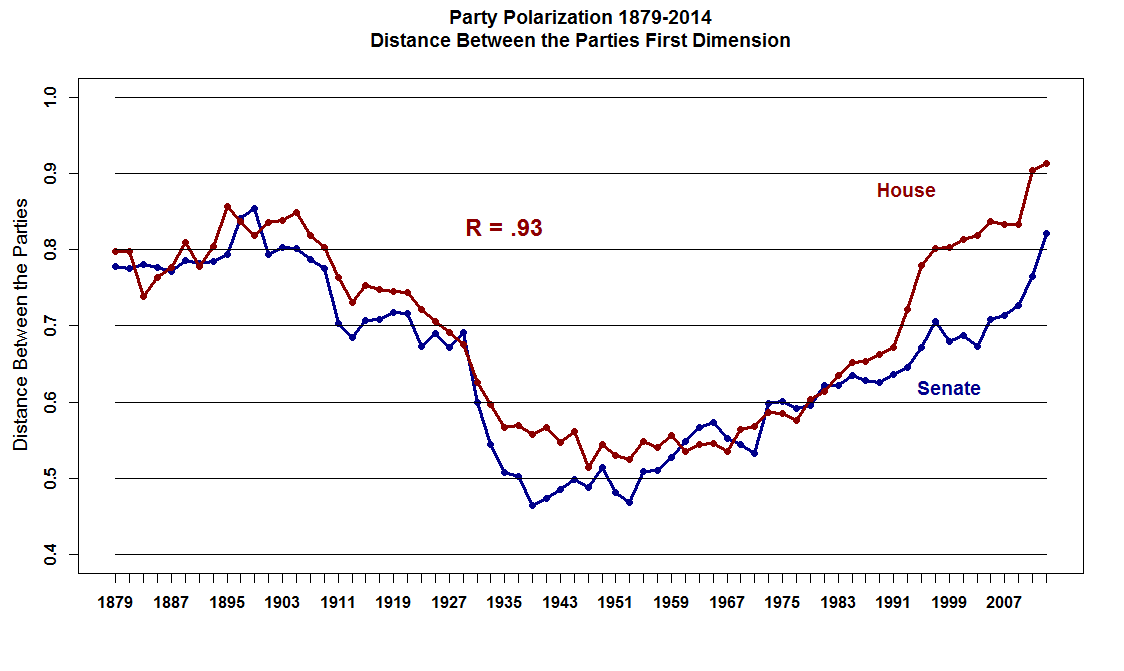
Below is a graph of the polarization of the House and Senate since the end of Reconstruction (1879-2014) using the joint space coordinates. Polarization is measured as the distance between the two major parties on the first, liberal-conservative dimension (see graph below). The pattern of polarization within the two chambers is almost the same with the 113^th House being the most polarized chamber since the end of Reconstruction.

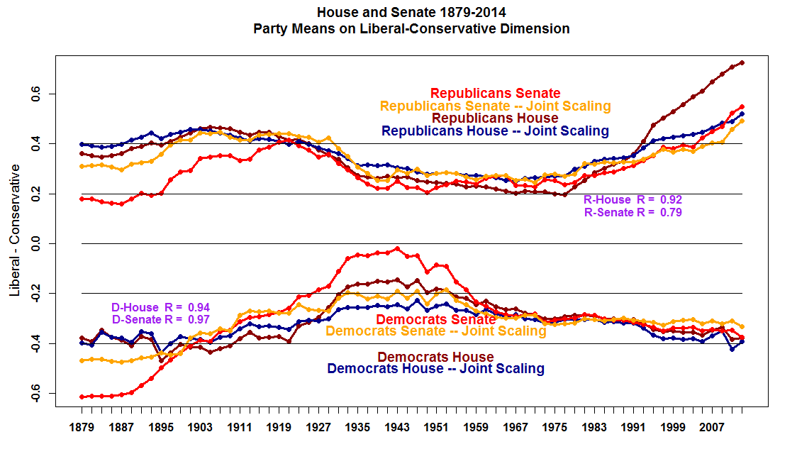
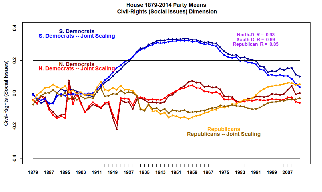
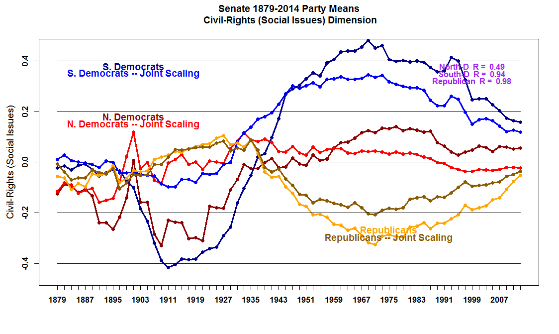
The three figures below show the Party Means for the current Post-Reconstruction Democrat-Republican two-party system. The figures pretty much speak for themselves. We have color coded the party lines and report correlations between the Party Means from the joint scaling versus the separate scalings. Note that for the graphs of the second dimension Party Means we separate out the Northern and Southern Democrats. The basic message of these graphs is that the Joint scaling is reproducing the Party trend lines during the whole Post-Reconstruction period.